
| sex | age | race | height | weight | actn3.r577x | ndrm.ch |
|---|---|---|---|---|---|---|
| Female | 20 | Caucasian | 60.0 | 90 | CT | 80.0 |
| Female | 21 | Caucasian | 68.0 | 149 | CT | 57.1 |
| Male | 18 | Caucasian | 74.0 | 183 | CT | 50.0 |
| Male | 24 | Other | 72.6 | 135 | TT | 85.7 |
| Male | 21 | Caucasian | 65.0 | 133 | CT | 40.0 |
| Male | 28 | Asian | 71.0 | 141 | CC | 42.9 |
| Female | 23 | Hispanic | 63.2 | 129 | TT | 30.0 |
A Biostatistics Primer
September 4, 2026
Welcome to HST 190!
What is this course about?
- Statistical reasoning is the process of drawing scientific conclusions from data in a rational, consistent way
- Goals for the course:
- develop an intuition for the key concepts that underpin the statistical analysis of data
- read the “Methods” section of an article, and understand/critique the approach taken
- learn to analyze and draw scientific conclusions from data
Overview of course logistics
- Ten “lecture” sessions, each 3 hours long
- Reading will be assigned prior to each lecture
- given the fast pace of the course, this is strongly encouraged
- Three problem sets
- include exercises in
R
- include exercises in
- During breaks in the middle we will:
- complete group exercises
- learn a bit of
Rprogramming - discuss course projects
- You will also work on a group project and present results during one of the class meetings
Data basics
Example: the FAMuSS study
The Functional SNPs Associated with Muscle Size and Strength (FAMuSS) study and data is introduced in OI Biostat, Section 1.2.2.
One goal of the study—examine the association of demographic, physiological and genetic characteristics with muscle strength.
- In simpler terms, study the “sports gene” ACTN3.
Four rows from FAMuSS data matrix
Types of Variables
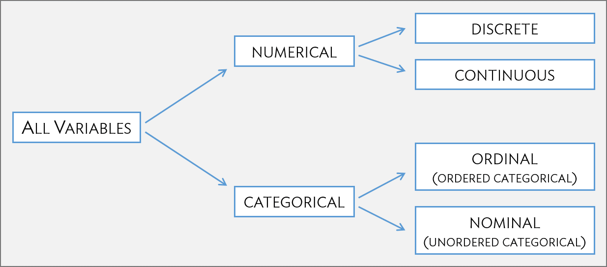
Numerical variables take on numerical values, such that numerical operations (sums, differences, etc.) are reasonable.
- Discrete: only take on integer values (e.g., # of family members)
- Continuous: take on any value in a specified range (e.g., height)
Categorical variables take on values that are names or labels; the possible values are called the variable’s levels.
- Ordinal: exists some natural ordering of levels (e.g., education)
- Nominal: no natural ordering of levels (e.g., gender)
Types of variables
Exploring data with simple tools
Techniques for exploring and summarizing data differ for numerical versus categorical variables.
Numerical and graphical summaries are useful for examining variables one at a time, but also for exploring the relationships between variables.
Numerical data
Distributions and summary measures
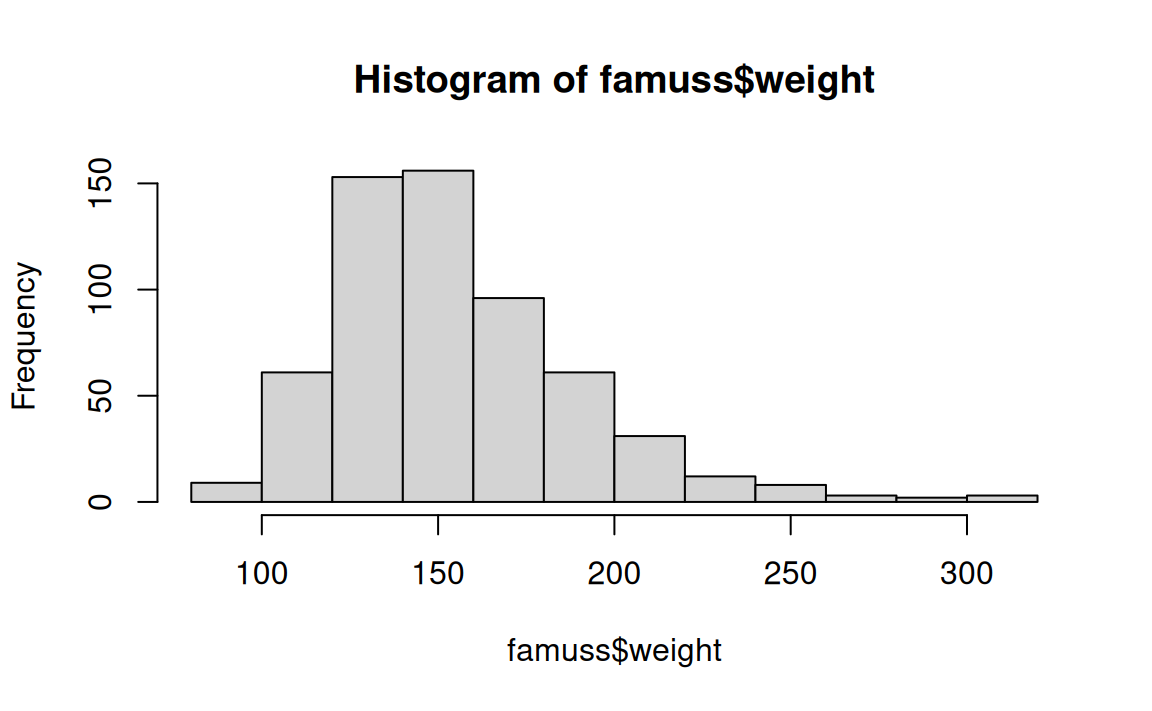
The collection of values for a numerical, continuous variable (e.g., weight) is the distribution of that variable.
Numerical and graphical summaries convey characteristics of a distribution without listing all the values.
Important characteristics include…
- Center: where is the middle of the distribution?
- Measures of center: mean, median
- Spread: how similar or varied are the values to each other?
- Measures of spread: standard deviation, interquartile range
Measures of center
The sample mean of a variable is the sum of all observations divided by the number of observations:
\[\overline{x} = \frac{x_1 + x_2 + \cdots + x_n}{n}\] where \(x_1, x_2, \ldots, x_n\) represent the \(n\) observed values in a sample.
The mean weight in the famuss dataset is 155.648 pounds.
Measures of center\(\ldots\)
The median is the value of the middle observation in a sample. If the number of observations is
- odd, then the median is the middle observation
- even, then the median is the average of the two middle observations
The median is the \(50^{\text{th}}\) percentile: 50% of observations lie below (and above) the median.
The median weight in the famuss dataset is 150 pounds.
Measures of spread
The variance and standard deviation measure the distance between a “typical” observation and the mean.
- An observation’s deviation is the distance between its value \(x\) and the sample mean \(\overline{x}\), that is \(d = x - \overline{x}\).
- Sample variance \(s^2\) is the sum of squared deviations divided by the number of observations, minus 1. \[s^2 = \frac{({x_1 - \overline{x})}^{2}+({x_2 - \overline{x})}^{2}+\cdots+({x_n - \overline{x})}^{2}}{n-1},\] where \(x_1, x_2, \dots, x_n\) represent the \(n\) observed values.
Measures of spread\(\ldots\)
The standard deviation is the distance between a “typical” observation and the mean, on the same unit scale.
- The standard deviation \(s\) is the square root of the variance \(s^2\). \[ s = \sqrt{\frac{({x_1 - \overline{x})}^{2} + ({x_2 - \overline{x})}^{2} + \cdots + ({x_n - \overline{x})}^{2}}{n-1}} \]
In the famuss dataset, the standard deviation of the variable weight is 34.59
Measures of Spread: Percentiles/Quartiles
The \(p^{\text{th}}\) percentile is the observation such that \(p\)% of the remaining observations fall below this observation.
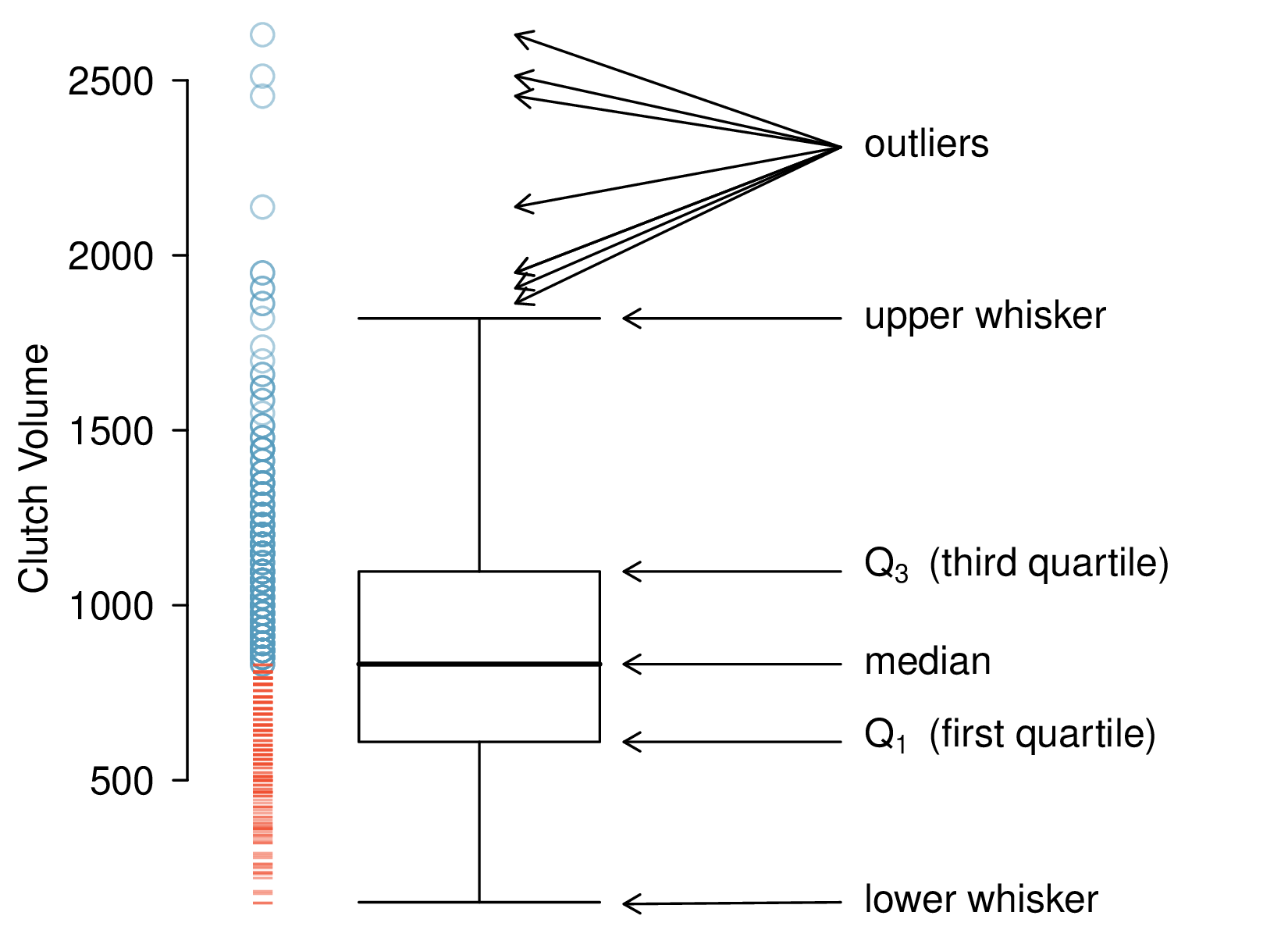
- The first quartile (\(Q_1\)) is the \(25^{\text{th}}\) percentile.
- The second quartile (\(Q_2\)), i.e., the median, is the \(50^{\text{th}}\) percentile.
- The third quartile (\(Q_3\)) is the \(75^{\text{th}}\) percentile.
Robust estimates
The median and IQR are often called robust estimates since they are less affected by extreme values than are means and standard deviations.
For distributions containing extreme observations, the median and IQR provide a more accurate sense of center and spread.
Histograms
Box-and-whisker plots
Vu and Harrington (2020), Figure 1.20 (frog data)
Categorical data
Tables
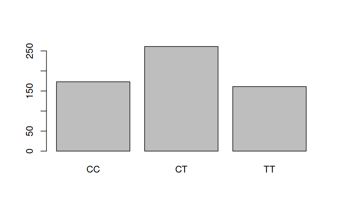
A table for a single variable, a frequency table or one-way table, summarizes the distribution of observations among categories.
Based on the table, describe the distribution of genotype at the location actn3.r577x among the study participants.
 CC  CT  TT
173 261 161
Bar plots for categorical data
A bar plot is a common way to display a single categorical variable.
Relationships between two variables
Two numerical variables
Two variables \(x\) and \(y\) are
- positively associated if \(y\) appears to increase as \(x\) appears to increase.
- negatively associated if \(y\) appears to decrease as \(x\) appears to increase.
Height and weight are positively associated.
A numerical variable and categorical variable\(\ldots\)
FAMuSS was designed to study the relationship between genotype at the location r577x in the gene ACTN3 and muscle strength.
Muscle strength was assessed by the percent change in non-dominant arm strength after resistance training (ndrm.ch).
What visualization would be a good choice to make this comparison?
Random variables
Basic Concepts About Random Variables
- Definition of a random variable
- Distributions of random variables
- Properties of operations on random variables
- expectation
- (co)variance
- standard deviation
Definition of a Random Variable
A random variable (RV) is a function that maps each event in a sample space \(\Omega\) to a number (e.g., in \(\R\)), i.e., \(X: \Omega \to \R\)
A discrete random variable takes on a finite number of values.
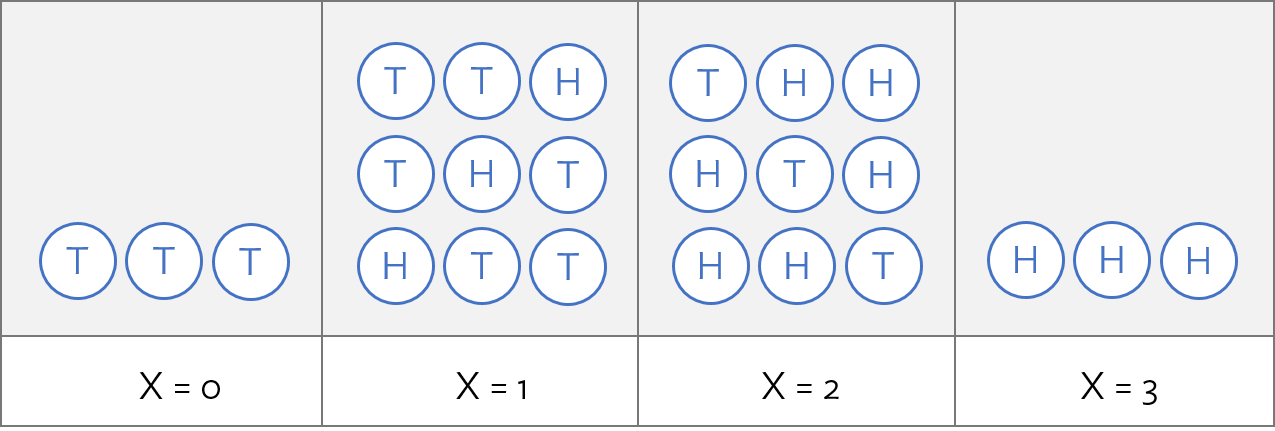
- Suppose \(X\) is the number of heads in 3 tosses of a fair coin.
- \(x\), a realization of \(X\), can take on the values 0, 1, 2, 3.
Distribution of a Discrete Random Variable
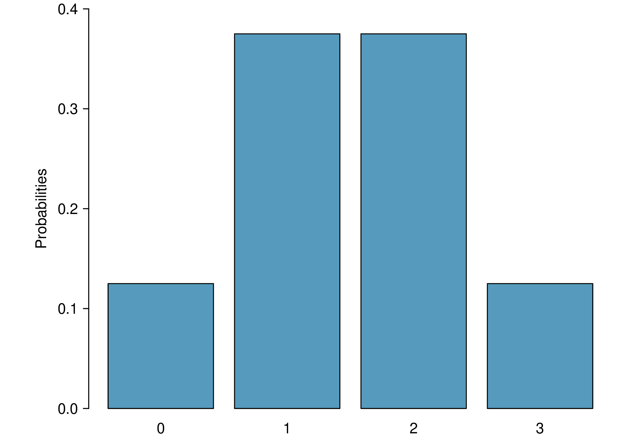
The distribution of a discrete RV is the collection of its values and the probabilities associated with those values.
The probability distribution for \(X\) is as follows:
| \(x_i\) | 0 | 1 | 2 | 3 |
|---|---|---|---|---|
| \(\Pr(X = x_i)\) | 1/8 | 3/8 | 3/8 | 1/8 |
For the distribution to be well-defined, we need that \[\sum_{x=0}^3 \Pr(X = x_i) = 1\]
Example Discrete Distribution of \(X\)
Expectation of a Random Variable
Let \(x_1, \ldots, x_k\) be realizations of \(X\) w/ corresponding probabilities \(\Pr(X=x_1), \ldots, \Pr(X=x_k)\), the expected value of \(X\) is the sum of each multiplied by its corresponding probability:
\[ \E(X) = x_1 \Pr(X=x_1) + \ldots + x_k \Pr(X=x_k) = \sum_{i=1}^{k}x_i \Pr(X=x_i) \]
Sometimes, \(\mu\) may be used in place of the notation \(\E(X)\) and may be written \(\mu_X\).
Calculating an Expectation
Returning to our coin tossing example,
\[\begin{align*} \E(X) &= 0 \Pr(X=0) + 1 \Pr(X=1) + 2 \Pr(X=2) + 3 \Pr(X = 3) \\ &= (0)(1/8) + (1)(3/8) + (2)(3/8) + (3)(1/8) \\ &= 12/8 \\ &= 1.5 \end{align*}\]
Linearity of Expectation
The expectation operator \(\E(X)\) is linear in that:
- \(\E(a \cdot X) = a \cdot \E(X)\), for a constant \(a\)
- \(\E(X + b) = \E(X) + b\), for a constant \(b\)
This turns out to be a very useful property. Intuitively, this follows from the expectation being summation (or integration) operation.
Variance of a Random Variable
Let \(x_1, \ldots, x_k\) be realizations of \(X\) w/ corresponding probabilities \(\Pr(X=x_1), \ldots, \Pr(X=x_k)\) and expected value \(\mu = \E(X)\), then the variance of \(X\), \(\text{Var}(X)\) (or \(\sigma^2_X\))1, is \[\begin{align*} \text{Var}(X) &= (x_1-\mu)^2 \Pr(X=x_1) + \ldots + (x_k-\mu)^2 \Pr(X=x_k) \\ &= \sum_{j=1}^{k} (x_j - \mu)^2 \Pr(X=x_j) \end{align*}\] The standard deviation of \(X\), written \(\text{SD}(X)\) (or \(\sigma_X\)), is just the square root of the variance.
Calculating the Variance of a Random Variable
Again returning to our coin tossing example,
\[\begin{align*} \sigma_X^2 &= (x_1-\mu_X)^2 \Pr(X=x_1) + \cdots+ (x_4-\mu)^2 \Pr(X=x_4) \\ &= (0 - 1.5)^2(1/8) + (1 - 1.5)^2 (3/8)\\ &\mspace{20mu} + (2 - 1.5)^2 (3/8) + (3 - 1.5)^2 (1/8) \\ &= 3/4 \notag \end{align*}\]
The standard deviation is \(\sqrt{3/4} = \sqrt{3}/2 =\) 0.866.
Variance and Expectation
Note that \(\text{Var}(X)\) is the expected squared distance1 of a given realization \(x\) from the RV \(X\)’s expected value \(\E[X]\), so \[\begin{align*} \text{Var}(X) &= \E[(X - \E[X])^2] \\ &= \cdots \\ &= \E[X^2] - \E[X]^2 \end{align*}\]
As noted before, if we define \(\tilde{X} \coloneqq X - \E(X)\), then we have \[\text{Var}(\tilde{X}) = \E(\tilde{X}^2)\]
Covariance of Two Random Variables
For two RVs, \(X\) and \(Y\), their covariance1, \(\text{Cov}(X,Y)\), measures the degree to which the two RVs vary together \[\begin{align*} \text{Cov}(X, Y) &= \E[(X - \E[X]) (Y - \E[Y])] \\ &= \cdots \\ &= \E[X Y] - \E[X] \E[Y] \end{align*}\]
The covariance is tied to another notion—correlation, which we will discuss later in a module on regression analysis.
Common distributions
Binomial Random Variables
A specific type of discrete RV is a binomial RV.
\(X\) is a binomial RV when it represents the number of successes in \(n\) independent replications1 of an experiment where
- Each replicate has two possible outcomes: success or failure
- The probability of success \(p\) in each replicate is constant
Binomial Random Variables
A binomial RV takes on values \(0, 1, 2, \ldots, n\). We use the shorthand \(X \sim \text{Bin}(n,p)\) to say that \(X\) follows a binomial distribution with \(n\) trials and \(p\) success probability.
For example, the number of heads in 3 tosses of a fair coin is a binomial RV with parameters \(n = 3\) and \(p = 0.5\).
For a binomial RV \(X \sim \text{Bin}(n,p)\) with parameters \(n\) and \(p\),
- \(\E[X] = np\)
- \(\text{Var}(X) = n p (1 - p)\)
Formula for the Binomial Distribution
Let \(x\) be the number of successes in \(n\) trials, then \[\Pr(x \text{ successes}) = \binom{\text{\# trials}} {\text{\# successes}} p^{\text{\# successes}}(1-p)^{\text{\# trials - \# successes}}\]
\[\Pr(X = x) = \binom{n}{x} p^x (1-p)^{n-x},\: x= 0, 1, 2, \dots, n\] Parameters of the distribution:
- \(n\) = number of trials
- \(p\) = probability of success
Calculating Binomial Probabilities in R
The function dbinom() is used to calculate \(\Pr(X = k)\).
dbinom(k, n, p): \(\Pr(X = k)\)
The function pbinom() is used to calculate \(\Pr(X \leq k)\) or \(\Pr(X > k)\).
pbinom(k, n, p): \(\Pr(X \leq k)\)pbinom(k, n, p, lower.tail = FALSE): \(\Pr(X > k)\)
Continuous Random Variables
A discrete random variable takes on a finite number of values.
- Number of heads in a \(n\) coin tosses
- Number of people who’ve had chicken pox in a random sample
A continuous random variable takes on any value in an interval.
- Height in a population
- Blood pressure in a population
Discrete RVs are counted, continuous RVs are measured.
Probabilities from Continuous Distributions
Two important features of continuous distributions:
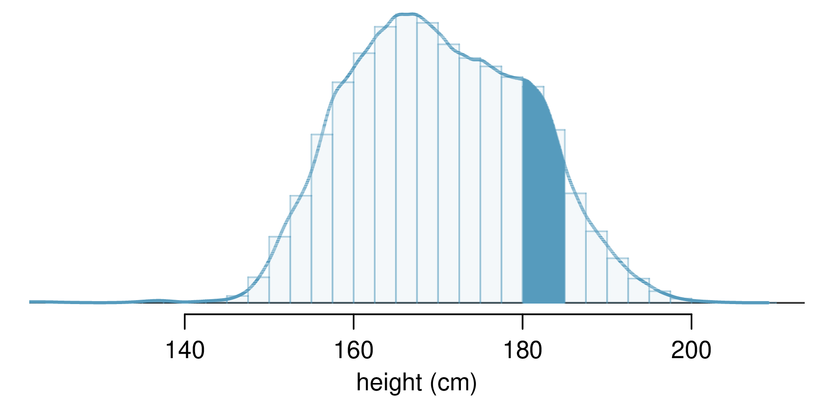
- The total area under the density curve is 1.
- The probability that a variable has a value within a specified interval is the area under the curve over that interval.
The “Empirical Rule” for the Normal Distribution
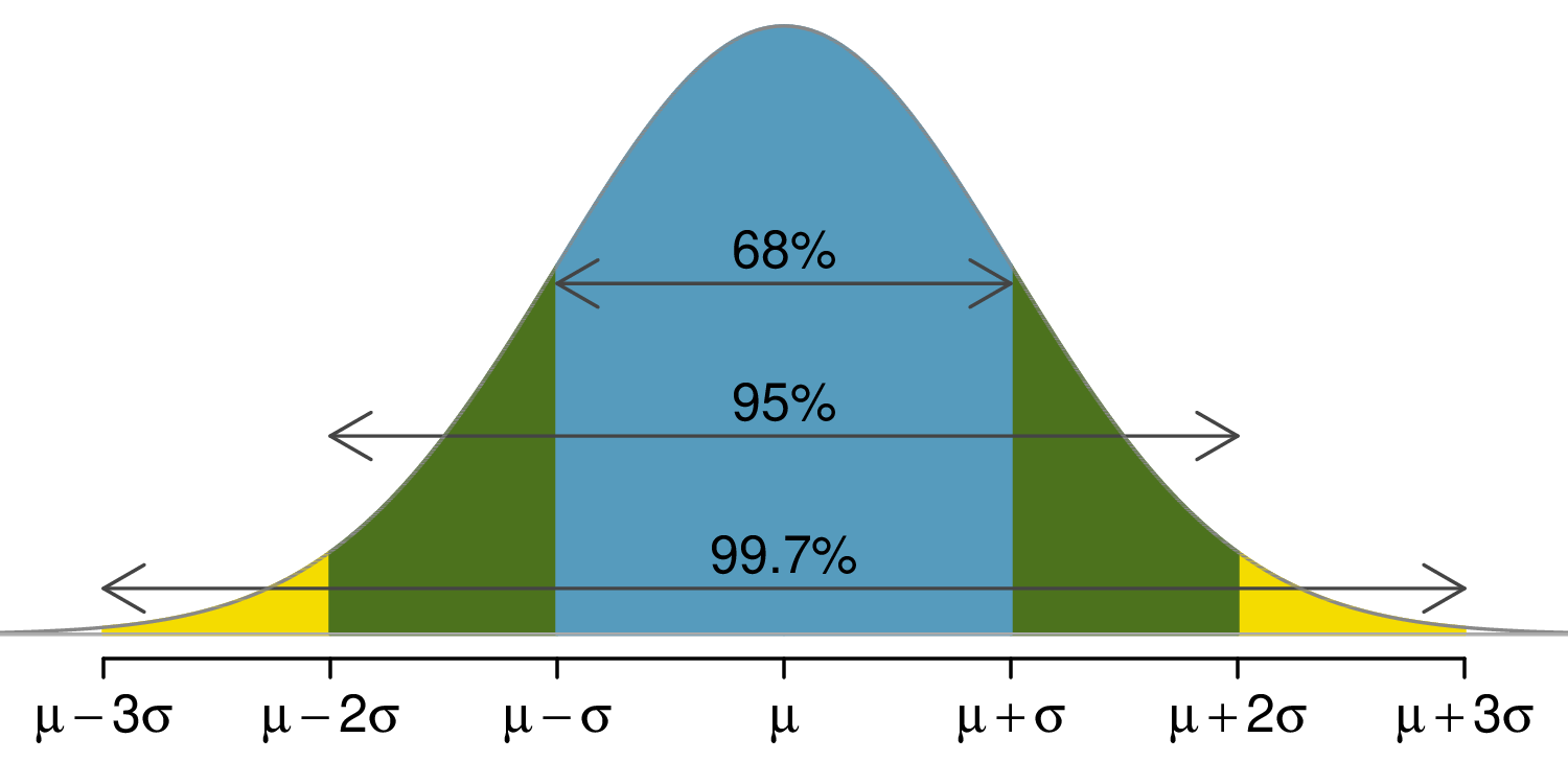
According to the “empirical rule,” for any1 normal distribution,
- approximately 68% of the data are within 1 SD of the mean
- approximately 95% of the data are within 2 SDs of the mean
- approximately 99.7% of the data are within 3 SDs of the mean
The “Empirical Rule” for the Normal Distribution
An Example of Using a Normal Distribution
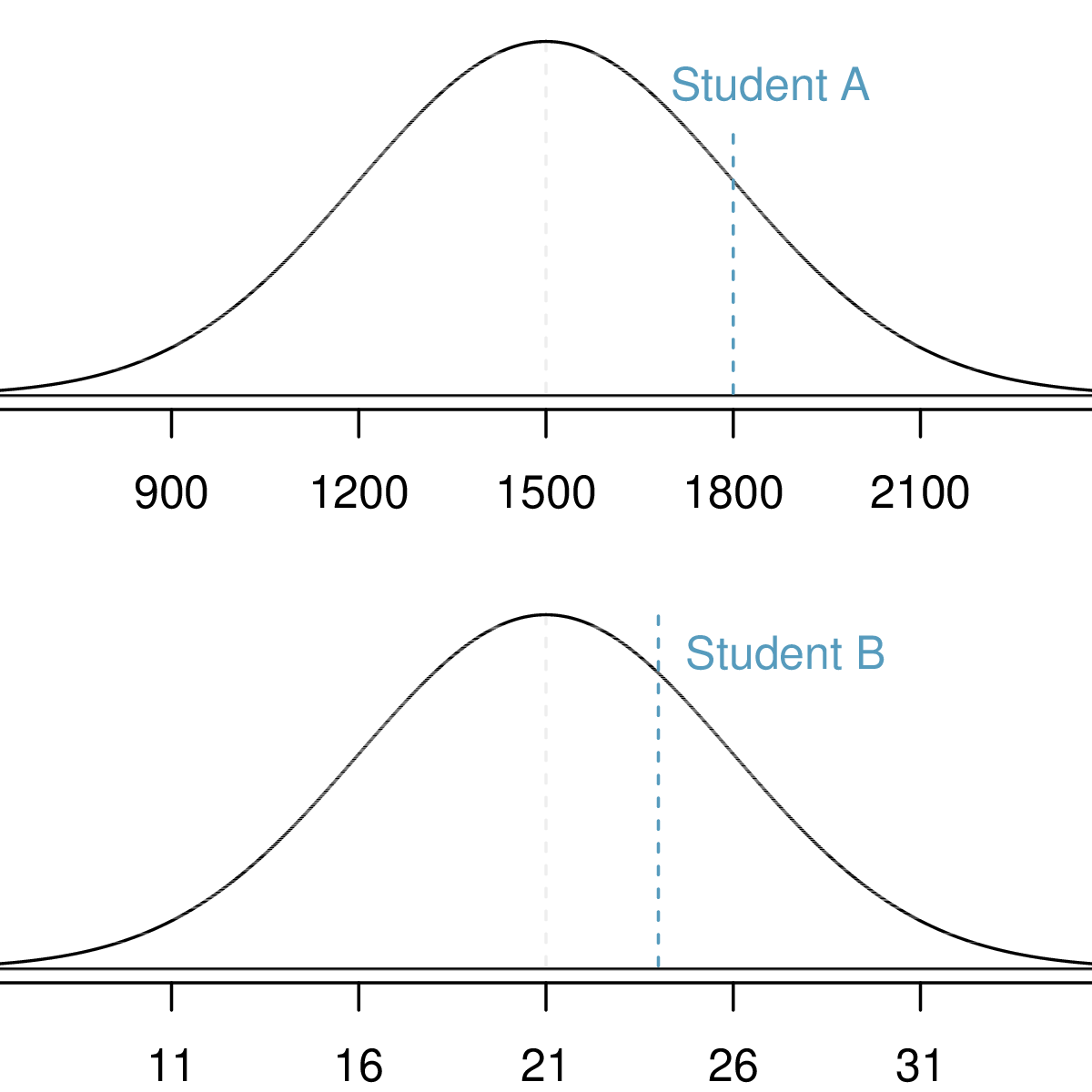
Assume that the distributions of test scores on the SAT and ACT are normal with means \(\mu_{\text{SAT}}\), \(\mu_{\text{ACT}}\) and variances \(\sigma^2_{\text{SAT}}\), \(\sigma^2_{\text{ACT}}\).
Suppose that one student scores an 1800 on the SAT (Student A) and another student scores a 24 on the ACT (Student B). Which student performed better?
Standard Normal Distribution
A standard normal distribution is defined as a normal distribution with mean 0 and variance 1. It is often denoted as \(Z \sim \text{N}(0, 1)\).
Any normal random variable \(X\) can be transformed into a standard normal random variable \(Z\).
\[Z = \dfrac{X - \mu}{\sigma} \qquad X = \mu + Z\sigma\]
Calculating Probabilities from Normal Distributions
What is the percentile rank for a student who scores an 1800 on the SAT for a year in which the scores are \(\text{N}(1500, 300)\)?
Calculate a \(Z\)-score. If \(X \sim \text{N}(\mu, \sigma^2)\), \(Z = \frac{X - \mu}{\sigma} \sim \text{N}(0, 1)\)
pnorm(z)gives the area (i.e., probability) to the left of \(z\)Alternatively, let
Rdo the work…
Words of Warning…
“Everyone is sure of this [that errors are normally distributed]…since the experimentalists believe that it is a mathematical theorem, and the mathematicians that it is an experimentally determined fact.” –Poincaré (1912)
“Far better an approximate answer to the right question, which is often vague, than the exact answer to the wrong question, which can always be made precise.” –Tukey (1962)
Summary Table of Distributions
| Binomial | Normal | Poisson | |
|---|---|---|---|
| Parameters | \(n\), \(p\) | \(\mu\), \(\sigma\) | \(\lambda\) |
| Possible values | \(0,1,\ldots,n\) | (-\(\infty\), \(\infty\)) | \(0,1,\ldots,\infty\) |
| Mean | \(np\) | \(\mu\) | \(\lambda\) |
| Standard Deviation | \(\sqrt{np(1-p)}\) | \(\sigma\) | \(\sqrt{\lambda}\) |
Appendix
Inner Product on a Vector Space
Recall that A vector is an ordered list of numbers, written \(x = (x_1, \ldots, x_n)\). Its norm (or “length”) generalizes the Pythagorean theorem:
\[\lVert x \rVert = \sqrt{x_1^2 + \cdots + x_n^2} \ ,\]
where, we say that the \(n\)-vector \(x\) has norm \(\lVert x \rVert\).
The inner product of two vectors multiplies them entry by entry and sums:
\[\langle x, y \rangle = x_1 y_1 + \cdots + x_n y_n\]
- A vector’s inner product with itself gives its squared length: \(\langle x, x \rangle = \lVert x \rVert^2\).
- The inner product measures how much two vectors point in the same direction. It is zero when they are orthogonal.
Covariance as an inner product
Consider mean-zero random variables \(X\) and \(Y\) treated as vectors. Then,
- \(\text{Cov}(X, Y)\) behaves exactly like \(\langle X, Y \rangle\) and
- \(\text{Var}(X) = \text{Cov}(X, X)\) behaves like \(\langle X, X \rangle = \lVert X \rVert^2\).
Here, standard deviation can be seen as a measure of length (and variance as squared distance); uncorrelated random variables are orthogonal vectors.
This explains a few seemingly unrelated facts:
- variance is a squared quantity
- standard deviation returns to the original units
- variance of a sum of uncorrelated variables is the sum of their variances
References
Poincaré, H. (1912) Calcul Des Probabilités. Gauthier-Villars.
Tukey, J. W. (1962) The future of data analysis. The Annals of Mathematical Statistics, 33, 1–67. Institute of Mathematical Statistics. DOI: 10.1214/aoms/1177704711.
Vu, J. and Harrington, D. (2020) Introductory Statistics for the Life and Biomedical Sciences. OpenIntro. Available at: https://openintro.org/book/biostat.

HST 190: Introduction to Biostatistics