
| sex | age | race | height | weight | actn3.r577x | ndrm.ch |
|---|---|---|---|---|---|---|
| Female | 20 | Caucasian | 60.0 | 90 | CT | 80.0 |
| Female | 21 | Caucasian | 68.0 | 149 | CT | 57.1 |
| Male | 18 | Caucasian | 74.0 | 183 | CT | 50.0 |
| Male | 24 | Other | 72.6 | 135 | TT | 85.7 |
| Male | 21 | Caucasian | 65.0 | 133 | CT | 40.0 |
| Male | 28 | Asian | 71.0 | 141 | CC | 42.9 |
| Female | 23 | Hispanic | 63.2 | 129 | TT | 30.0 |
Biostatistical Science and Data Analysis
September 3, 2025
Welcome to HST 190!
What is this course about?
- Statistical reasoning is the process of drawing scientific conclusions from data in a rational, consistent way
- Goals for the course:
- develop an intuition for the key concepts that underpin the statistical analysis of data
- read the “Methods” section of an article, and understand/critique the approach taken
- learn to analyze and draw scientific conclusions from data
Overview of course logistics
- Ten “lecture” sessions, each 3 hours long
- Reading will be assigned prior to each lecture
- given the fast pace of the course, this is strongly encouraged
- Three problem sets
- include exercises in
R
- include exercises in
- During breaks in the middle we will:
- complete group exercises
- learn a bit of
Rprogramming - discuss course projects
- You will also work on a group project and present results during one of the class meetings
Data basics
Example: the FAMuSS study
The Functional SNPs Associated with Muscle Size and Strength (FAMuSS) study and data is introduced in OI Biostat, Section 1.2.2.
One goal of the study—examine the association of demographic, physiological and genetic characteristics with muscle strength.
- In simpler terms, study the “sports gene” ACTN3.
Four rows from FAMuSS data matrix
Data basics
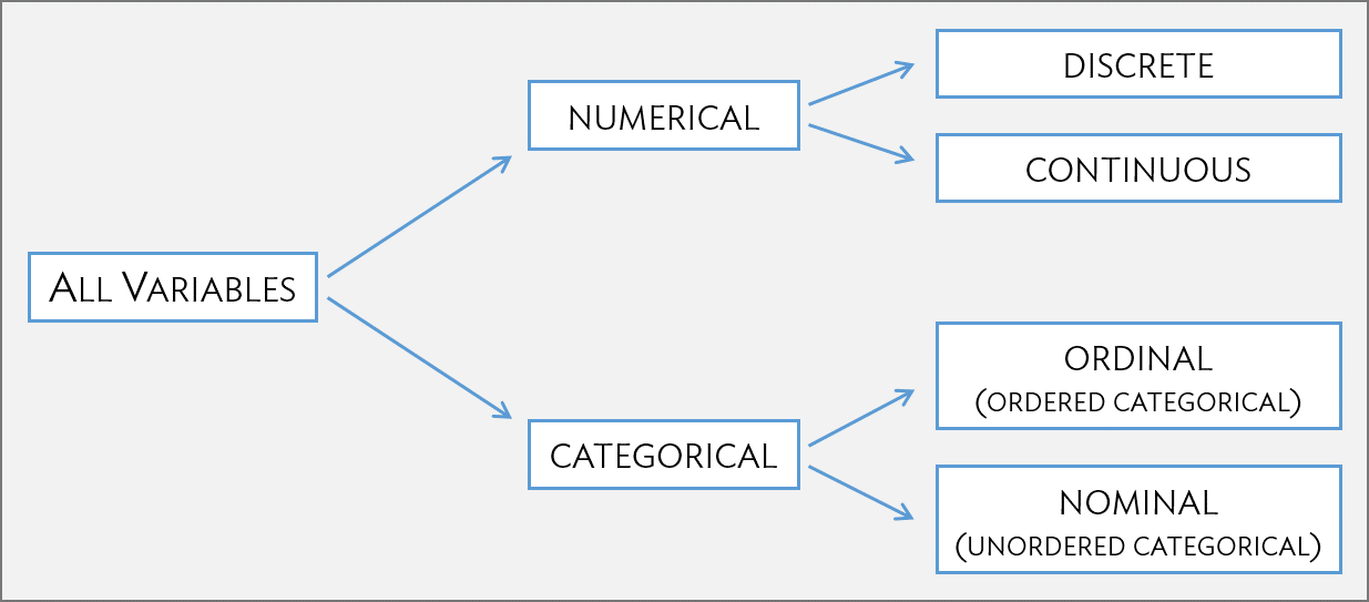
Types of Variables
Numerical variables take on numerical values, such that numerical operations (sums, differences, etc.) are reasonable.
- Discrete: only take on integer values (e.g., # of family members)
- Continuous: take on any value in a specified range (e.g., height)
Categorical variables take on values that are names or labels; the possible values are called the variable’s levels.
- Ordinal: exists some natural ordering of levels (e.g., education)
- Nominal: no natural ordering of levels (e.g., gender)
Types of variables
Exploring data with simple tools
Techniques for exploring and summarizing data differ for numerical versus categorical variables.
Numerical and graphical summaries are useful for examining variables one at a time, but also for exploring the relationships between variables.
Numerical data
Distributions and summary measures
The collection of values for a numerical, continuous variable (e.g., weight) is the distribution of that variable.
Numerical and graphical summaries convey characteristics of a distribution without listing all the values.
Important characteristics include…
- Center: where is the middle of the distribution?
- Measures of center: mean, median
- Spread: how similar or varied are the values to each other?
- Measures of spread: standard deviation, interquartile range
Measures of center
The sample mean of a variable is the sum of all observations divided by the number of observations:
\[\overline{x} = \frac{x_1 + x_2 + \cdots + x_n}{n}\] where \(x_1, x_2, \ldots, x_n\) represent the \(n\) observed values in a sample.
The mean weight in the famuss dataset is 155.648 pounds.
Measures of center\(\ldots\)
The median is the value of the middle observation in a sample. If the number of observations is
- odd, then the median is the middle observation
- even, then the median is the average of the two middle observations
The median is the \(50^{\text{th}}\) percentile: 50% of observations lie below (and above) the median.
The median weight in the famuss dataset is 150 pounds.
Measures of spread
The variance and standard deviation measure the distance between a “typical” observation and the mean.
- An observation’s deviation is the distance between its value \(x\) and the sample mean \(\overline{x}\), that is \(d = x - \overline{x}\).
- Sample variance \(s^2\) is the sum of squared deviations divided by the number of observations, minus 1. \[s^2 = \frac{({x_1 - \overline{x})}^{2}+({x_2 - \overline{x})}^{2}+\cdots+({x_n - \overline{x})}^{2}}{n-1},\] where \(x_1, x_2, \dots, x_n\) represent the \(n\) observed values.
Measures of spread\(\ldots\)
The standard deviation is the distance between a “typical” observation and the mean, on the same unit scale.
- The standard deviation \(s\) is the square root of the variance \(s^2\). \[ s = \sqrt{\frac{({x_1 - \overline{x})}^{2} + ({x_2 - \overline{x})}^{2} + \cdots + ({x_n - \overline{x})}^{2}}{n-1}} \]
In the famuss dataset, the standard deviation of the variable weight is 34.59
Measures of Spread: Percentiles/Quartiles
The \(p^{\text{th}}\) percentile is the observation such that \(p\)% of the remaining observations fall below this observation.
- The first quartile (\(Q_1\)) is the \(25^{\text{th}}\) percentile.
- The second quartile (\(Q_2\)), i.e., the median, is the \(50^{\text{th}}\) percentile.
- The third quartile (\(Q_3\)) is the \(75^{\text{th}}\) percentile.
Measures of Spread: Percentiles/Quartiles\(\ldots\)
The interquartile range (IQR) is the distance between the third and first quartiles: \(IQR = Q_3 - Q_1\)
In the famuss dataset, the IQR for the variable weight is 42
Robust estimates
The median and IQR are often called robust estimates since they are less affected by extreme values than are means and standard deviations.
For distributions containing extreme observations, the median and IQR provide a more accurate sense of center and spread.
Histograms

Histograms\(\ldots\)
Histograms show important features of the shape of a distribution:
- Symmetry, or lack of it (skew)
- Minimum and maximum values
- Regions of high frequency (modes)
Histograms are not so good for:
- Displaying the median or quartiles
- Showing subtle skewing
- Identifying extreme values
Box-and-whisker plots
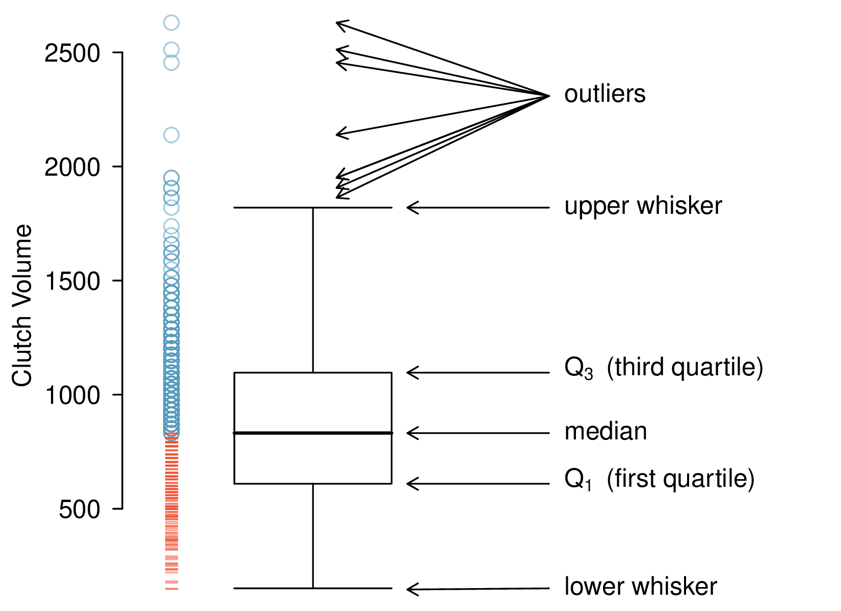
Vu and Harrington (2020), Figure 1.20 (frog data)
Boxplots
A boxplot indicates the first, second, and third quartiles of a distribution
It also identifies potential outliers – observations far from the center
- Large outliers are > \(Q_3 + (1.5\times \text{IQR})\)
- Small outliers are < \(Q_1 - (1.5 \times \text{IQR})\)
On a boxplot\(\ldots\)
- The rectangle extends from the first quartile to the third quartile, with a line at the second quartile (median).
- Whiskers capture data that fall between \(Q_1 - (1.5 \times IQR)\) and \(Q_3 + (1.5 \times IQR)\), and they must end at data points.
- Potential outliers are dotted.
Categorical data
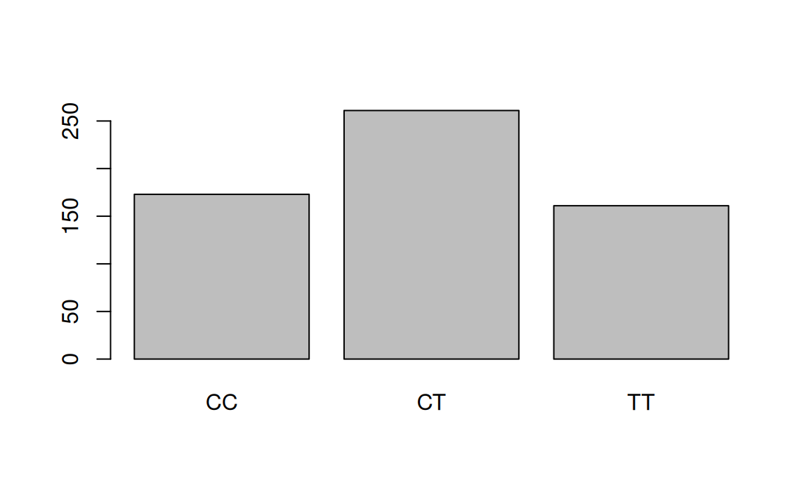
Tables
A table for a single variable, a frequency table or one-way table, summarizes the distribution of observations among categories.
Based on the table, describe the distribution of genotype at the location actn3.r577x among the study participants.
 CC  CT  TT
173 261 161
Bar plots for categorical data
A bar plot is a common way to display a single categorical variable.
Relationships between two variables
Summarizing relationships between two variables
Approaches for summarizing relationships between two variables vary depending on variable types…
- Two numerical variables
- Two categorical variables
- One numerical variable and one categorical variable
Two numerical variables
Two variables \(x\) and \(y\) are
- positively associated if \(y\) increases as \(x\) increases.
- negatively associated if \(y\) decreases as \(x\) increases.
Height and weight are positively associated.
Two numerical variables \(\ldots\)

Two numerical variables\(\ldots\)
Correlation is a numerical summary that measures the strength of a linear relationship between two variables.
- Introduced in Vu and Harrington (2020) Section 1.6.1; details in Ch. 6 (on regression).
- The correlation coefficient \(r\) takes on values between -1 and 1.
- The closer \(r\) is to \(\pm 1\), the stronger the linear association.
In the famuss dataset, the correlation \(r\) between height and weight is 0.5309
Two categorical variables \(\ldots\)
Relative risk (RR) is one way of summarizing data presented in a two-way table of study outcome by participant group.
\[\text{RR} = \frac{\mathbb{P}(Y = 1 \mid X = \text{exposed})}{\mathbb{P}(Y = 1 \mid X = \text{unexposed})}\]
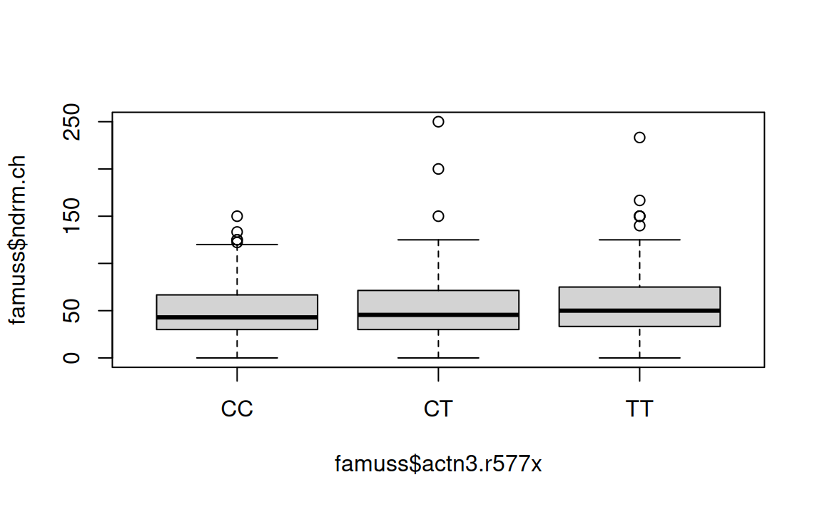
A numerical variable and categorical variable\(\ldots\)
FAMuSS was designed to study the relationship between genotype at the location r577x in the gene ACTN3 and muscle strength.
Muscle strength was assessed by the percent change in non-dominant arm strength after resistance training (ndrm.ch).
What visualization would be a good choice to make this comparison?
A numerical variable and categorical variable\(\ldots\)
References
Vu, Julie, and David Harrington. 2020. Introductory Statistics for the Life and Biomedical Sciences. OpenIntro. https://openintro.org/book/biostat.

HST 190: Introduction to Biostatistics