Concepts in Probability

September 3, 2025
Basic Concepts of Probability
Intro to Probability
People often colloquially refer to probability…
- “What are the chances the Red Sox will win this weekend?”
- “What’s the chance of rain tomorrow?”
- “What is the chance that a patient responds to a new therapy?”
Formalizing concepts and terminology around probability theory is essential for better understanding probability (and statistics).
Random Experiments
A random experiment is an action or process that leads to one of several possible outcomes.
- For example, flipping a coin leads to two possible outcomes: either heads or tails.
The probability of an outcome is the proportion of times that the outcome would occur if the random phenomenon could be observed an infinite number of times.
- If a fair coin is flipped an infinite number of times, heads would be obtained 50% of the time.
Outcomes and events
An outcome in a study is the result observable once the experiment has been conducted.
- The sum of the faces on two dice that have been rolled.
- The response of a patient treated with an experimental therapy.
An event is a collection of outcomes.
- The sum after rolling two dice is 7.
- 22 of 30 patients in a study have a good response to a therapy.
Events can be referred to by letters. For example, if \(A\) is the event of rolling a number smaller than 3 on a die, then \(A = \{1, 2 \}\).
Disjoint (Mutually Exclusive) Events
Two events or outcomes are called disjoint or mutually exclusive if they cannot both happen at the same time.

Here, \(A\) and \(B\) being disjoint means
- \(\Pr(A \cup B) = \Pr(A) + \Pr(B) = 2/6 + 2/6 = 4/6\)
- The probability of rolling a 1, 2, 4, or 6 on a six-sided die is 4/6.
Addition Rule for Disjoint Events
If \(A\) and \(B\) are two disjoint events, then the probability that either occurs is \(\Pr(A \cup B) = \Pr(A) + \Pr(B)\)1.
If there are \(k\) disjoint events \(A_1,\dots,A_k\), the probability that one of these outcomes will occur is \(\Pr(A_1) + \Pr(A_2) + \cdots + \Pr(A_k)\)
General Addition Rule
Suppose that we are interested in the probability of drawing a diamond or a face card out of a standard 52-card deck.
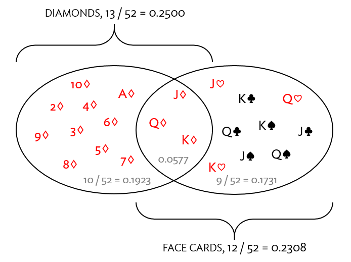
Does \(\Pr(\text{diamond or face card}) = 13/52 + 12/52\)?
General Addition Rule…
No, we need to correct the double counting of the three cards that are in both events, subtract the probability that both events occur… \[\begin{align*} \Pr(\text{diamond or face}) =& \Pr(\text{diamond}) + \Pr(\text{face}) - \Pr(\text{diamond and face}) \\ =& 13/52 + 12/52 - 3/52 \\ =& 22/52 \end{align*}\]
Thus, for any two events \(A\) and \(B\), the probability that either occurs is \(\Pr(A \cup B) = \Pr(A) + \Pr(B) - \Pr(A \cap B)\)1.
Sample Space
A sample space is an exhaustive list of mutually exclusive outcomes.
Suppose the possible \(k\) outcomes are denoted \(O_1, O_2, \dots, O_k\). The sample space can be expressed as \(S = \{O_1, O_2, \dots, O_k\}\).
Given a sample space \(S = \{O_1, O_2, \dots, O_k\}\), the sum of the probabilities of each outcome must equal 1 – that is, \[\sum_{i=1}^{k}P(O_i)=1\]
Complement of an Event
Let \(D = \{2, 3\}\) represent the event that the outcome of a single die roll is 2 or 3.
The complement of \(D\) represents all possible outcomes within the sample space that are not in \(D\).
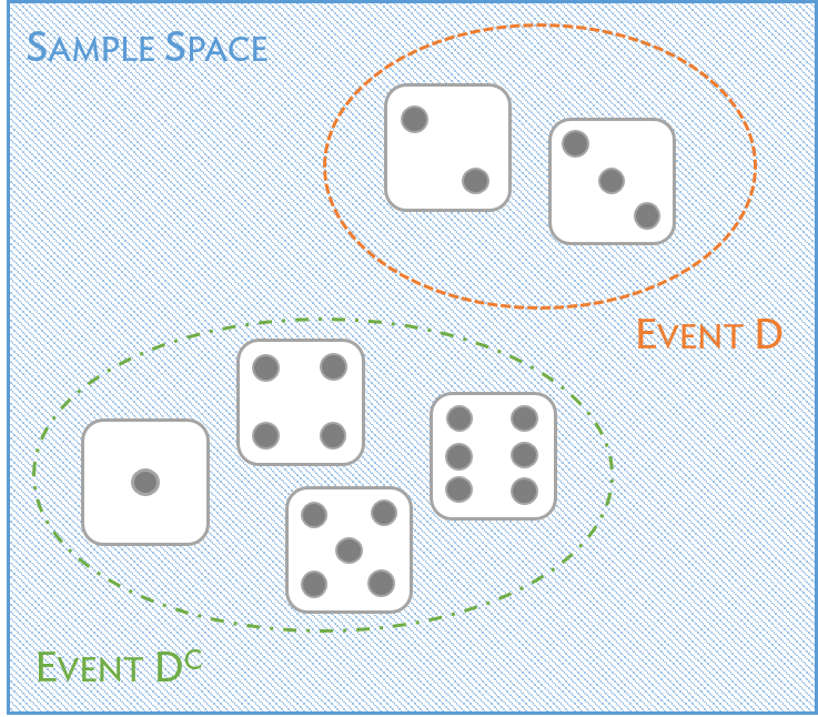
Complement of an Event…
The complement of an event \(A\) is denoted by \(A^C\).
An event and its complement are mathematically related:
\[\Pr(A) + \Pr(A^C) = 1 \qquad \Pr(A) = 1 - \Pr(A^C)\]
Independent Events
Two events \(A\) and \(B\) are independent if the probability that both \(A\) and \(B\) is the product of their probabilities: \(\Pr(A \cap B) = \Pr(A)\Pr(B)\)
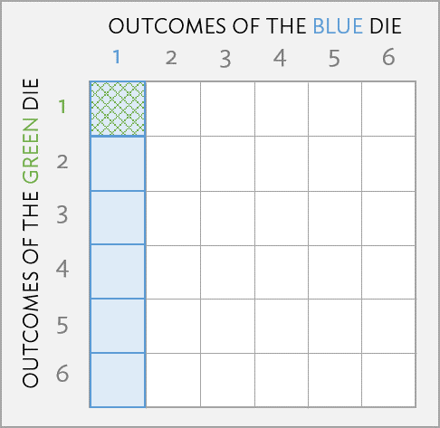
A blue die and a green die are rolled. What is the probability of rolling two 1’s?
Conditional Probability
An example from childhood mortality
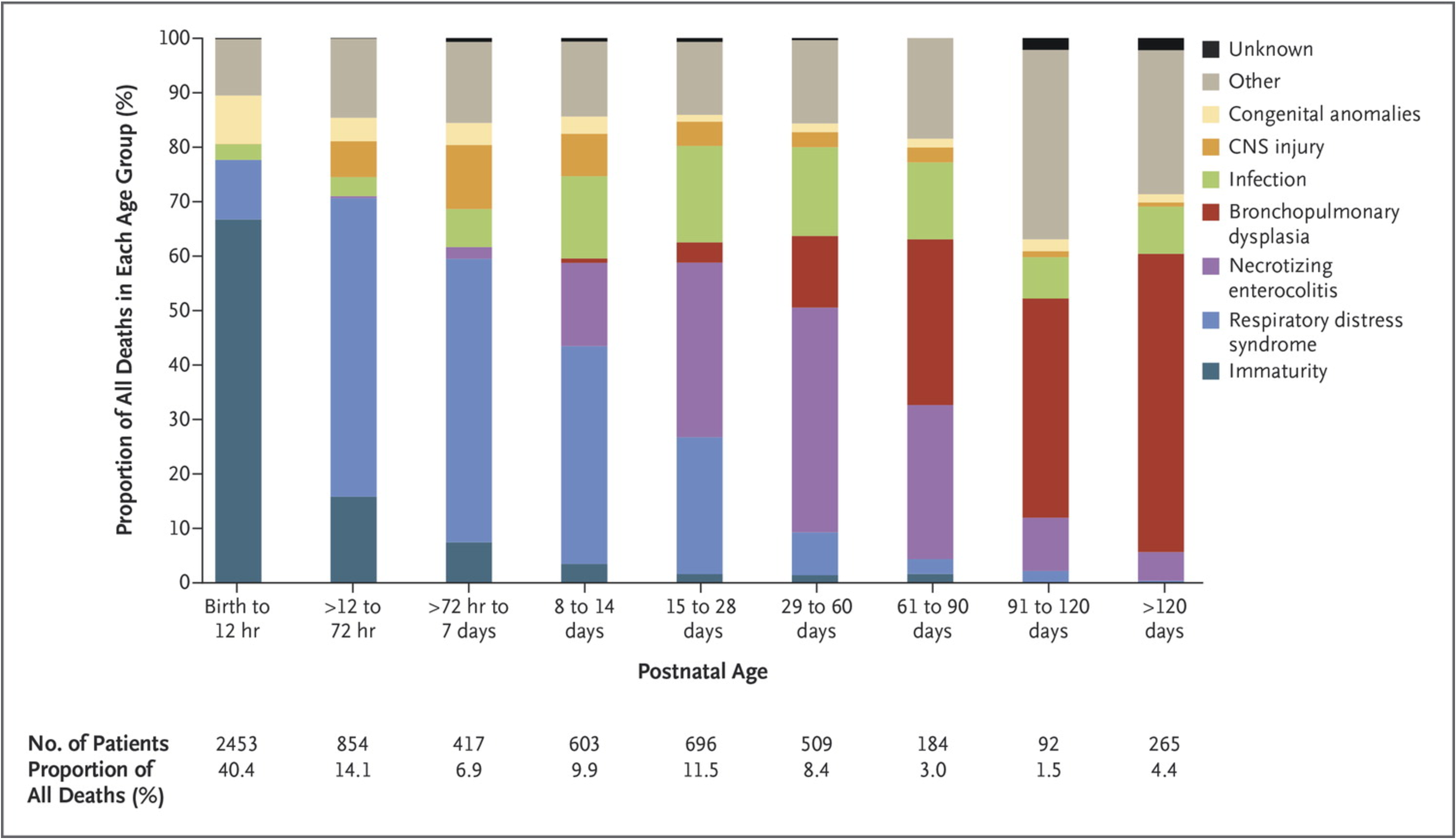
Published in Patel, et al., NEJM (2015) Vol 372, pp 331 - 340.
Conditional Probability: Intuition
Consider height in the US population.
What is the probability that a randomly selected individual in the population is taller than 6 feet, 4 inches?
- Suppose you learn that the selected individual is a professional basketball player.
- Does this change the probability that the individual is taller than 6 feet, 4 inches? Yes or no, and why?
Conditional Probability: Concept
The conditional probability of an event \(A\), given a second event \(B\), is the probability of \(A\) happening, knowing that \(B\) has happened. This conditional probability is denoted \(\Pr(A \mid B)\).
Toss a fair coin three times. Let \(A\) be the event that exactly two heads occur, and \(B\) the event that at least two heads occur.
- Conditioning on \(B\) means that the sample space consists of \(\{HHH, HHT, HTH, THH\}\) – all possible sets of three tosses where at least two heads occurred.
- In this restricted set of outcomes, \(A\), consists of the last three, so \(\Pr(A \mid B) = 3/4\).
Conditional Probability: Formal Definition
As long as \(\Pr(B) > 0\), then \(\Pr(A \mid B) = \dfrac{\Pr(A \cap B)}{\Pr(B)}\).
From the definition, \[\begin{align*} \Pr(A \mid B) =& \dfrac{\Pr(\text{at least two heads and exactly two heads})}{\Pr(\text{at least two heads})} \\ =& \dfrac{\Pr(\text{exactly two heads})}{\Pr(\text{at least two heads})} \\ =& \dfrac{3/8}{4/8} = 3/4 \end{align*}\]
Independence, Again…
A consequence of the definition of conditional probability:
- If \(\Pr(A \mid B) = \Pr(A)\), then \(A\) and \(B\) are independent; knowing \(B\) offers no information about whether \(A\) occurred.
Thus, independence means that conditioning has no effect since the two event spaces do not overlap.
General Multiplication Rule
If \(A\) and \(B\) are two events, then \(\Pr(A \cap B) = \Pr(A \mid B) \Pr(B)\).
Rearranging the definition of conditional probability yields this \[\Pr(A \mid B) = \frac{\Pr(A \cap B)}{\Pr(B)} \rightarrow \Pr(A \mid B) \Pr(B) = \Pr(A \cap B)\]
Unlike the previously mentioned multiplication rule, this is valid for events that might not be independent.
Positive Predictive Value and Bayes’ Theorem
Pre-natal Testing for Trisomy 21, 13, and 18
Some congenital disorders are caused by an additional copy of a chromosome being attached to another in reproduction.
- Trisomy 21: Down syndrome, approximately 1 in 800 births
- Trisomy 13: Patau’s syndrome, physical and mental disabilities, approximately 1 in 16,000 newborns
- Trisomy 18: Edward’s syndrome, nearly always fatal, either in stillbirth or infant mortality, occurs in about 1 in 6,000 births
Cell-free fetal DNA (cfDNA), copies of embryo DNA present in maternal blood, can be used as a non-invasive test.
Cell-free Fetal DNA-based Testing
Initial testing of the technology was done using archived samples of genetic material in children whose trisomy status was known.
The results are variable, but generally very good:
- Of 1000 unborn children with one of the disorders, about 980 have cfDNA that tests positive. The test has high sensitivity (true positive rate).
- Of 1000 unborn children without the disorders, about 995 test negative. The test has high specificity (true negative rate).
Cell-free Fetal DNA-based Testing…
The designers of a diagnostic test strive for accuracy: A test should have high sensitivity and specificity.
A family with an unborn child undergoing testing wants to know the likelihood of the condition being present if the test is positive.
Suppose a child has tested positive for trisomy 21. What is the probability the child does have trisomy 21, given the positive test result?
Defining Events in Diagnostic Testing
Events of interest in diagnostic testing:
- \(D\) = {disease present}
- \(D^C\) = {disease absent}
- \(T^+\) = {positive test result}
- \(T^-\) = {negative test result}
Could use \(T\) and \(T^C\), but \(T^+\) and \(T^-\) are consistent with notation in medical and public health literature.
Characteristics of a Diagnostic Test
The following measures are all characteristics of a diagnostic test.
- Sensitivity = \(\Pr(T^+ \mid D)\)
- Specificity = \(\Pr(T^- \mid D^C)\)
- False negative rate = \(\Pr(T^- \mid D)\)
- Note that \(\Pr(T^- \mid D) = 1 - P (T^+ \mid D)\), i.e., 1 - sensitivity
- False positive rate = \(\Pr(T^+ \mid D^C)\)
- Note that \(\Pr(T^+ \mid D^C) = 1 - \Pr(T^- \mid D^C)\), that is, 1 - specificity
Positive Predictive Value of a Test
Suppose an individual tests positive for a disease.
The positive predictive value (PPV) of a diagnostic test is the probability that the disease is present, given the test returns a positive results: PPV = \(\Pr(D \mid T^+)\)
The characteristics of a diagnostic test include \(\Pr(T^+ \mid D)\), among other probabilities, but not the reverse conditional \(\Pr(D \mid T^+)\).
Bayes’ Theorem (or Bayes’ Rule)
Bayes’ Theorem (simplest form): \(\Pr(A \mid B) = \frac{\Pr(B \mid A) \Pr(A)} {\Pr(B)}\)
Follows directly from the definition of conditional probability, noting that \(\Pr(A) \Pr(B \mid A)\) equals \(\Pr(A \text{ and } B)\):
\[\Pr(A \mid B) = \frac{\Pr(A \cap B)}{\Pr(B)} = \frac{\Pr(B \mid A) \Pr(A)} {\Pr(B)}\]
The Denominator \(\Pr(B)\) in Bayes’ Theorem
Bayes’ Theorem is usually stated differently, since, in many problems, \(\Pr(B)\) is not given directly but is calculated via a general multiplication rule:
Suppose \(A\) and \(B\) are events. Then, \[\begin{align*} \Pr(B) = & \Pr(B \cap A) + \Pr(B \cap A^C) \\ = & \Pr(B \mid A) \Pr(A) + \Pr(B \mid A^C) \Pr(A^C) \end{align*}\]
Bayes’ Theorem can be written as: \(\Pr(A \mid B) = \frac{\Pr(A) \Pr(B \mid A)}{\Pr(B)} = \frac{\Pr(B \mid A) \Pr(A)}{\Pr(B \mid A) \Pr(A) + \Pr(B \mid A^C) \Pr(A^C)}\)
Bayes’ Theorem for Diagnostic Tests
\[\begin{align*} \Pr(D \mid T^+) = & \dfrac{\Pr(D \cap T^{+})}{\Pr(T^+)} \\ =& \dfrac{\Pr(D \cap T^{+})}{\Pr(D \cap T^{+}) + \Pr(D^C \cap T^{+})} \\ =& \frac{\Pr(T^{+} \mid D) \Pr(D)}{\Pr(T^{+} \mid D) \Pr(D) + \Pr(T^{+} \mid D^{C}) \Pr(D^C)} \\ =& \frac{\text{sensitivity} \times \text{prevalence}}{[\text{sensitivity} \times \text{prevalence}] + [(\text{1 - specificity}) \times (\text{1 - prevalence})]} \end{align*}\]
Bayes’ Theorem for Diagnostic Tests…
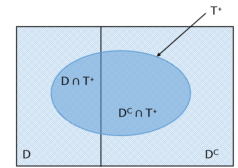
\[ \Pr(D \mid T^+) = \dfrac{\Pr(D \cap T^{+})}{\Pr(T^+)} = \dfrac{\Pr(D \cap T^{+})}{\Pr(D \cap T^{+}) + \Pr(D^C \cap T^{+})} \]

HST 190: Introduction to Biostatistics