HST 190 at HMS – Random Variables and Probability Distributions

Basic Concepts About Random Variables

Definition of a random variable
Distributions of random variables
Properties of operations on random variables
- expectation
- (co)variance
- standard deviation

Definition of a Random Variable

A random variable (RV) is a function that maps each event in a sample space $Ω$ to a number (e.g., in $R$ ), i.e., $X : Ω \to R$

A discrete random variable takes on a finite number of values.

Suppose $X$ is the number of heads in 3 tosses of a fair coin.
$x$ , a realization of $X$ , can take on the values 0, 1, 2, 3.

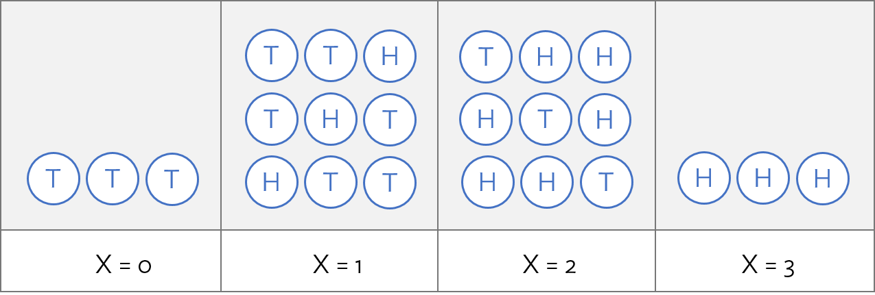
Distribution of a Discrete Random Variable

The distribution of a discrete RV is the collection of its values and the probabilities associated with those values.

The probability distribution for $X$ is as follows:

$x_{i}$	0	1	2	3
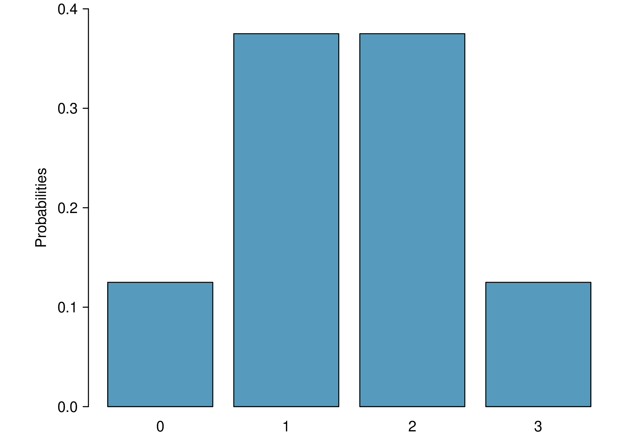
$P (X = x_{i})$	1/8	3/8	3/8	1/8

For the distribution to be well-defined, we need that $\sum_{x = 0}^{3} P (X = x_{i}) = 1$

Example Discrete Distribution of $X$

Expectation of a Random Variable

Let $x_{1}, \dots, x_{k}$ be realizations of $X$ w/ corresponding probabilities $P (X = x_{1}), \dots, P (X = x_{k})$ , the expected value of $X$ is the sum of each multiplied by its corresponding probability:

$E (X) = x_{1} P (X = x_{1}) + \dots + x_{k} P (X = x_{k}) = \sum_{i = 1}^{k} x_{i} P (X = x_{i})$

Sometimes, $μ$ may be used in place of the notation $E (X)$ and may be written $μ_{X}$ .

Calculating an Expectation

Returning to our coin tossing example,

$\begin{aligned} E (X) & = 0 P (X = 0) + 1 P (X = 1) + 2 P (X = 2) + 3 P (X = 3) \\ = (0) (1 / 8) + (1) (3 / 8) + (2) (3 / 8) + (3) (1 / 8) \\ = 12 / 8 \\ = 1.5 \end{aligned}$

Linearity of Expectation

The expectation operator $E (X)$ is linear in that:

$E (a \cdot X) = a \cdot E (X)$ , for a constant $a$
$E (X + b) = E (X) + b$ , for a constant $b$

This turns out to be a very useful property. Intuitively, this follows from the expectation being summation (or integration) operation.

Variance of a Random Variable

Let $x_{1}, \dots, x_{k}$ be realizations of $X$ w/ corresponding probabilities $P (X = x_{1}), \dots, P (X = x_{k})$ and expected value $μ = E (X)$ , then the variance of $X$ , $Var (X)$ (or $σ_{X}^{2}$ )¹, is $\begin{aligned} Var (X) & = (x_{1} - μ)^{2} P (X = x_{1}) + \dots + (x_{k} - μ)^{2} P (X = x_{k}) \\ = \sum_{j = 1}^{k} (x_{j} - μ)^{2} P (X = x_{j}) \end{aligned}$ The standard deviation of $X$ , written $SD (X)$ (or $σ_{X}$ ), is just the square root of the variance.

Calculating the Variance of a Random Variable

Again returning to our coin tossing example,

$\begin{aligned} σ_{X}^{2} & = (x_{1} - μ_{X})^{2} P (X = x_{1}) + \dots + (x_{4} - μ)^{2} P (X = x_{4}) \\ = (0 - 1.5)^{2} (1 / 8) + (1 - 1.5)^{2} (3 / 8) \\ + (2 - 1.5)^{2} (3 / 8) + (3 - 1.5)^{2} (1 / 8) \\ = 3 / 4 \end{aligned}$

The standard deviation is $\sqrt{3 / 4} = \sqrt{3} / 2 =$ 0.866.

Variance and Expectation

Note that $Var (X)$ is the expected squared distance¹ of a given realization $x$ from the RV $X$ ’s expected value $E [X]$ , so $\begin{aligned} Var (X) & = E [(X - E [X])^{2}] \\ = \dots \\ = E [X^{2}] - E [X]^{2} \end{aligned}$

As noted before, if we define $\tilde{X} : = X - E (X)$ , then we have $Var (\tilde{X}) = E ({\tilde{X}}^{2})$

Covariance of Two Random Variables

For two RVs, $X$ and $Y$ , their covariance¹, $Cov (X, Y)$ , measures the degree to which the two RVs vary together $\begin{aligned} Cov (X, Y) & = E [(X - E [X]) (Y - E [Y])] \\ = \dots \\ = E [X Y] - E [X] E [Y] \end{aligned}$

The covariance is tied to another notion—correlation, which we will discuss later in a module on regression analysis.

Binomial Random Variables

A specific type of discrete RV is a binomial RV.

$X$ is a binomial RV when it represents the number of successes in $n$ independent replications¹ of an experiment where

Each replicate has two possible outcomes: success or failure
The probability of success $p$ in each replicate is constant

Binomial Random Variables

A binomial RV takes on values $0, 1, 2, \dots, n$ . We use the shorthand $X \sim Bin (n, p)$ to say that $X$ follows a binomial distribution with $n$ trials and $p$ success probability.

For example, the number of heads in 3 tosses of a fair coin is a binomial RV with parameters $n = 3$ and $p = 0.5$ .

For a binomial RV $X \sim Bin (n, p)$ with parameters $n$ and $p$ ,

$E [X] = n p$
$Var (X) = n p (1 - p)$

The Binomial Coefficient

The binomial coefficient $(\binom{n}{x})$ is the number of ways to choose $x$ items from a set of size $n$ , where the order of the choice is ignored.

Mathematically, $(\binom{n}{x}) = \frac{n!}{x! (n - x)!}$

$n = 1, 2, \dots$
$x = 0, 1, 2, \dots, n$
For any integer $m$ , $m! = (m) (m - 1) (m - 2) \dots (1)$

Formula for the Binomial Distribution

Let $x$ be the number of successes in $n$ trials, then $P (x successes) = (\binom{# trials}{# successes}) p^{# successes} (1 - p)^{# trials - # successes}$

$P (X = x) = (\binom{n}{x}) p^{x} (1 - p)^{n - x}, x = 0, 1, 2, \dots, n$ Parameters of the distribution:

$n$ = number of trials
$p$ = probability of success

Calculating Binomial Probabilities in `R`

The function dbinom() is used to calculate $P (X = k)$ .

dbinom(k, n, p): $P (X = k)$

The function pbinom() is used to calculate $P (X \leq k)$ or $P (X > k)$ .

pbinom(k, n, p): $P (X \leq k)$
pbinom(k, n, p, lower.tail = FALSE): $P (X > k)$

Continuous Random Variables

A discrete random variable takes on a finite number of values.

Number of heads in a $n$ coin tosses
Number of people who’ve had chicken pox in a random sample

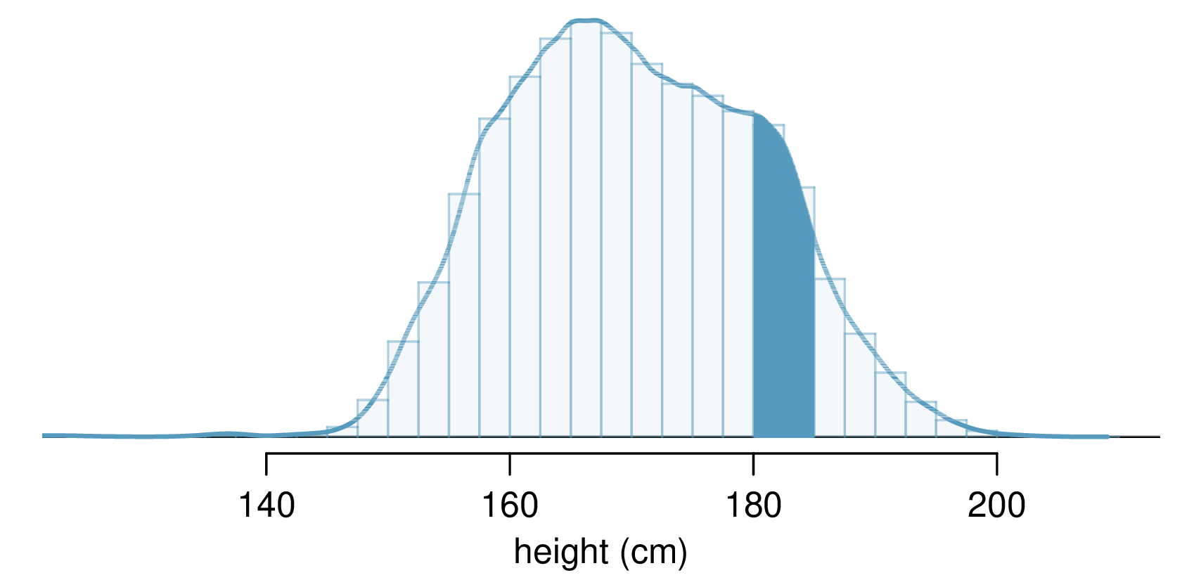
A continuous random variable takes on any value in an interval.

Height in a population
Blood pressure in a population

Discrete RVs are counted, continuous RVs are measured.

Probabilities from Continuous Distributions

Two important features of continuous distributions:

The total area under the density curve is 1.
The probability that a variable has a value within a specified interval is the area under the curve over that interval.

Probabilities from Continuous Distributions

When working with continuous random variables, probability is found for intervals of values rather than individual values.

Formally, the probability that a continuous RV $X$ takes on any single individual value is zero, that is, $P (X = x) = 0$ ¹.
Thus, $P (a < X < b)$ is equivalent to $P (a \leq X \leq b)$ .

The “Empirical Rule” for the Normal Distribution

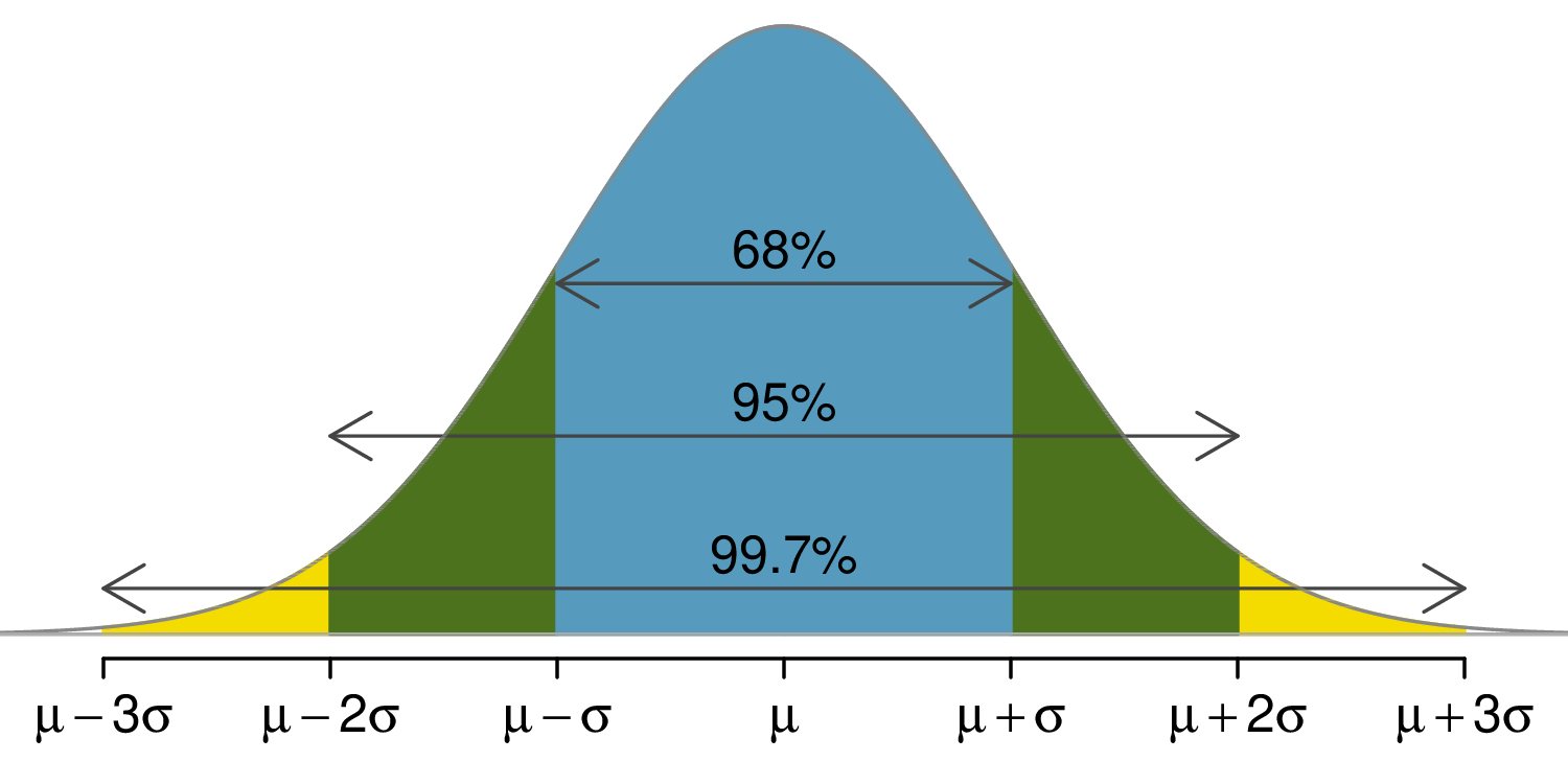
According to the “empirical rule,” for any¹ normal distribution,

approximately 68% of the data are within 1 SD of the mean
approximately 95% of the data are within 2 SDs of the mean
approximately 99.7% of the data are within 3 SDs of the mean

The “Empirical Rule” for the Normal Distribution

An Example of Using a Normal Distribution

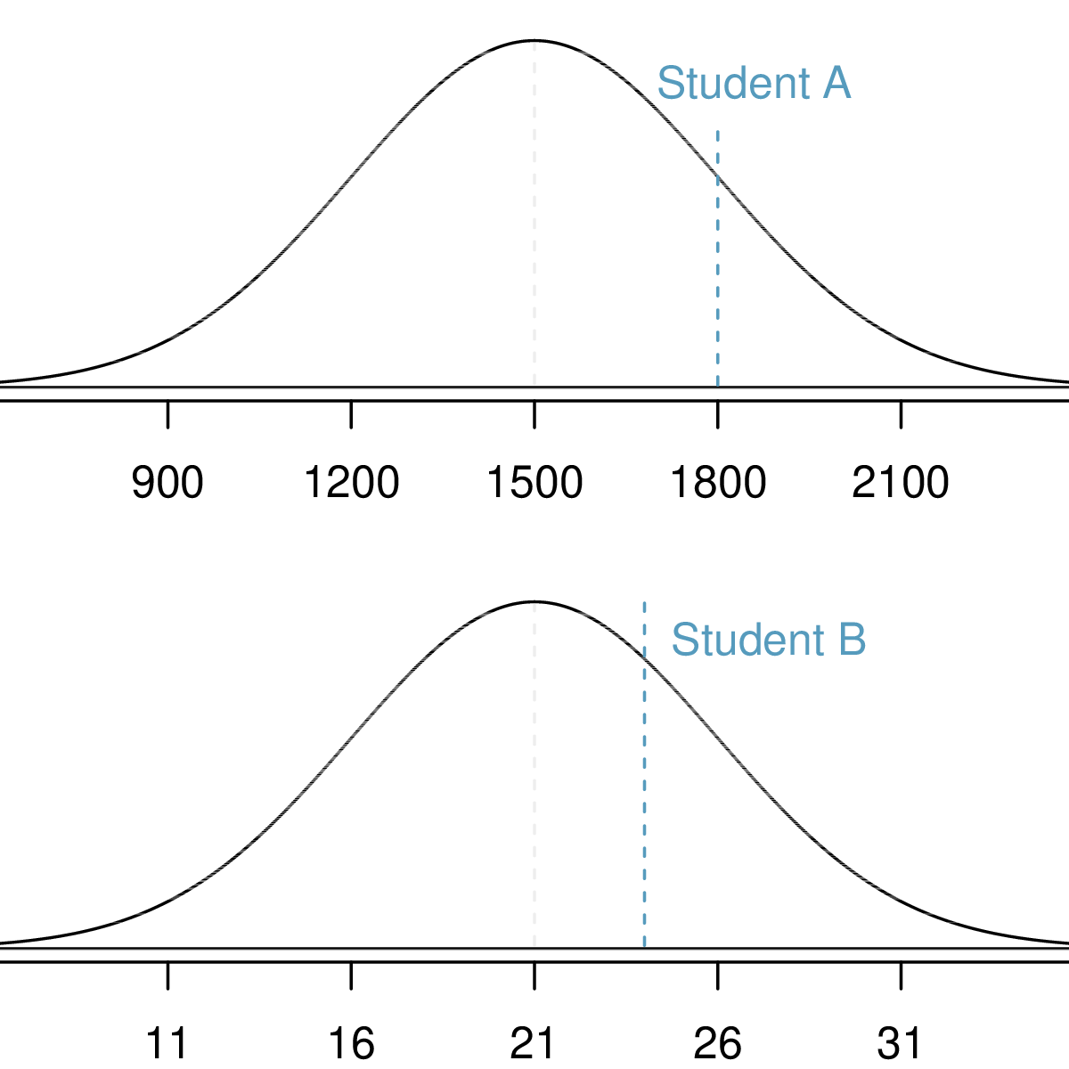
Assume that the distributions of test scores on the SAT and ACT are normal with means $μ_{SAT}$ , $μ_{ACT}$ and variances $σ_{SAT}^{2}$ , $σ_{ACT}^{2}$ .

Suppose that one student scores an 1800 on the SAT (Student A) and another student scores a 24 on the ACT (Student B). Which student performed better?

Standard Normal Distribution

A standard normal distribution is defined as a normal distribution with mean 0 and variance 1. It is often denoted as $Z \sim N (0, 1)$ .

Any normal random variable $X$ can be transformed into a standard normal random variable $Z$ .

$Z = \frac{X - μ}{σ} X = μ + Z σ$

Example of Using a Normal Distribution

SAT scores are $N (1500, 300)$ ; ACT scores are $N (21, 5)$ .
$x_{A}$ is the score of Student A; $x_{B}$ is the score of Student B.

$Z_{A} = \frac{x_{A} - μ_{S A T}}{σ_{S A T}} = \frac{1800 - 1500}{300} = 1$

$Z_{B} = \frac{x_{B} - μ_{A C T}}{σ_{A C T}} = \frac{24 - 21}{5} = 0.6$

Calculating Probabilities from Normal Distributions

What is the percentile rank for a student who scores an 1800 on the SAT for a year in which the scores are $N (1500, 300)$ ?

Calculate a $Z$ -score. If $X \sim N (μ, σ^{2})$ , $Z = \frac{X - μ}{σ} \sim N (0, 1)$
pnorm(z) gives the area (i.e., probability) to the left of $z$
```
pnorm(1)
```
```
[1] 0.8413447
```
Alternatively, let R do the work…
```
pnorm(1800, 1500, 300)
```
```
[1] 0.8413447
```

Calculating Probabilities from Normal Distributions

What score on the SAT would put a student in the 99^th percentile?

Identify the $Z$ -value. qnorm(p) calculates the value $z$ (a quantile) such that for a $Z \sim N (0, 1)$ , $p = P (Z \leq z)$ .
```
qnorm(0.99)
```
```
[1] 2.326348
```
If $Z \sim N (0, 1)$ , then $X = σ Z + μ$ , and $X \sim N (μ, σ^{2})$ , so $X = σ Z + μ = 300 (2.33) + 1500 = 2199$
Alternatively, let R do the work …
```
qnorm(0.99, 1500, 300)
```
```
[1] 2197.904
```

Words of Warning…

“Everyone is sure of this [that errors are normally distributed]…since the experimentalists believe that it is a mathematical theorem, and the mathematicians that it is an experimentally determined fact.” –Poincaré (1912)

“Far better an approximate answer to the right question, which is often vague, than the exact answer to the wrong question, which can always be made precise.” –Tukey (1962)

The Poisson Distribution

The Poisson distribution is used to calculate probabilities for rare events that accumulate over time (but is often used for counts).

It used most often in settings where events happen at a rate $λ$ per unit of population and per unit time, such as the annual incidence of a disease in a population.

Typical example: for children ages 0-14, the incidence rate of acute lymphocytic leukemia (ALL) was about 30 diagnosed cases per million children per year in the decade 2000-2010.
Always important to note and understand the units.

Example: Outbreaks of Childhood Leukemia

Fortunately, childhood cancers are rare.

For children ages 0-14, the incidence rate of acute lymphocytic leukemia (ALL) was approximately 30 diagnosed cases per million children per year in the decade from 2000-2010. Given that about 20% of the US population are in this age range, we may ask

What is the incidence rate of ALL over a 5 year period?
In a small city of 75,000 people, what is the probability of observing exactly 8 cases of ALL over a 5 year period?
In the small city, what is the probability of observing 8 or more cases of ALL over a 5 year period?

Poisson Distribution

Suppose events occur over a fixed time window in such a way that

The probability an event occurs in an interval is proportional to the length of the interval.
Events occur independently at a rate $λ$ per unit of time.

Poisson Distribution

Then the probability of exactly $x$ events in one unit of time is $P (X = x) = \frac{e^{- λ} λ^{x}}{x!}, x = 0, 1, 2, \dots$

The mean is $λ$ , i.e., $E [X] = λ$ .
The standard deviation is $\sqrt{λ}$ , i.e., $Var (X) = λ$ .

Poisson Distribution

The probability of exactly $x$ events $t$ units of time is $P (X = x) = \frac{e^{- λ t} (λ t)^{x}}{x!}, x = 0, 1, 2, \dots$

The mean is $λ t$ , i.e., $E [X] = λ t$ .
The standard deviation is $\sqrt{λ t}$ , i.e., $Var (X) = λ t$ .

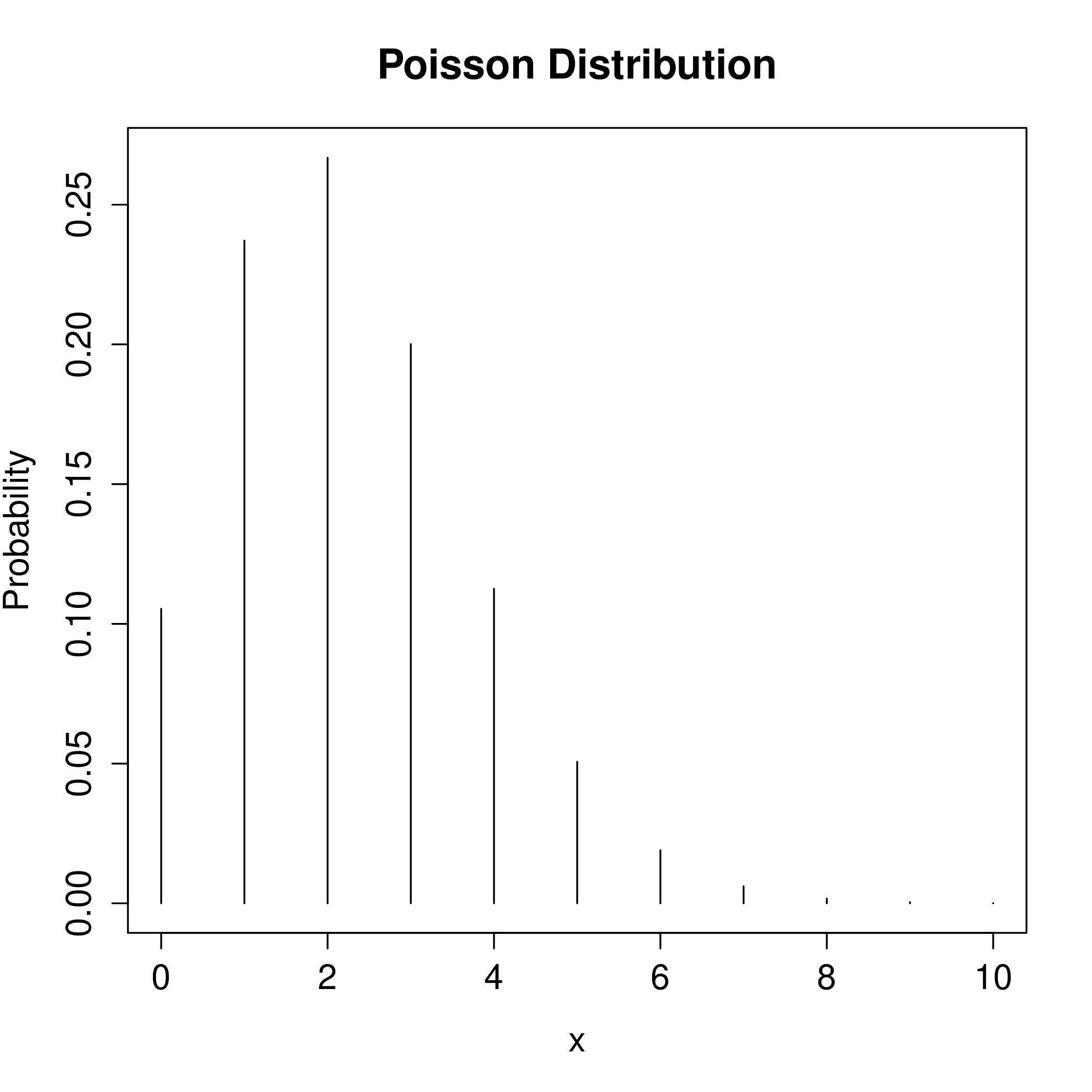
Poisson Distribution with $λ = 2.25$

Childhood Leukemia Incidence

See Example 3.37 of Vu and Harrington (2020) for details.

What is the incidence rate of ALL over a 5 year period?

Incidence rate of ALL in a year is 30 cases per 1,000,000 children: $\frac{30}{1, 000, 000} = 0.00003 = 3 \times 10^{- 5}$

Incidence rate in a 5-year period is (5)(30) per 1,000,000 children: $\frac{150}{1, 000, 000} = 0.00015 = 1.5 \times 10^{- 4}$

…and what about a city of size 75,000?

In a small city of 75,000 people, what is the probability of observing exactly 8 cases of ALL over a 5 year period?

In a city of 75,000 people, about $(75, 000) (0.20) = 15, 000$ children will be age 0-14.

The five-year rate of new cases for the whole city would be

$(1.5 \times 10^{- 4}) (15, 000) = 2.25$

What is the probability of 8 cases over 5 years?

In a small city, what is the probability of observing 8 or more ALL cases in a 5-year period?

$P (X = 8) = \frac{e^{- λ} λ^{x}}{x!} = \frac{e^{(- 2.25)} (2.25)^{8}}{8!}$

Easiest to calculate this in R. To do so, suppose $X \sim Pois (λ)$ , then dpois(k, lambda) gives $P (X = k)$

dpois(8, lambda = 2.25)

[1] 0.001717027

…but what is the probability of 8 or more cases?

In a small city, what is the probability of observing 8 or more ALL cases in a 5 year period?

Would 8 or more cases be a rare event? Suppose $X \sim Pois (λ)$ and calculate $P (X \geq 8) = 1 - P (X \leq 7)$ .

Compute $P (X \leq k)$ using ppois(k, lambda)

1 - ppois(7, lambda = 2.25)

[1] 0.002267088

Or $P (X > k)$ as ppois(k, lambda, lower.tail = FALSE)

ppois(7, lambda = 2.25, lower.tail = FALSE)

[1] 0.002267088

Summary Table of Distributions

	Binomial	Normal	Poisson
Parameters	$n$ , $p$	$μ$ , $σ$	$λ$
Possible values	$0, 1, \dots, n$	(- $\infty$ , $\infty$ )	$0, 1, \dots, \infty$
Mean	$n p$	$μ$	$λ$
Standard Deviation	$\sqrt{n p (1 - p)}$	$σ$	$\sqrt{λ}$

References

Poincaré, Henri. 1912. Calcul Des Probabilités. Vol. 1. Gauthier-Villars.

Tukey, John W. 1962. “The Future of Data Analysis.” The Annals of Mathematical Statistics 33 (1): 1–67. https://doi.org/10.1214/aoms/1177704711.

Vu, Julie, and David Harrington. 2020. Introductory Statistics for the Life and Biomedical Sciences. OpenIntro. https://openintro.org/book/biostat.