HST 190 at HMS – Elements of Statistical Inference, Part I

Statistical inference?

Statistics uses tools from probability and data analysis to

draw inferences about populations from samples
quantify uncertainty (or confidence) about an inference

We’ll illustrate inferential principles in the setting of

estimating average characteristics of a well-defined population
drawing conclusions about that characteristic

Perspectives on statistical inference

Some pithy philosophy on statistics

Statisticians are “engaged in an exhausting but exhilarating struggle with the biggest challenge that philosophy makes to science: how do we translate information into knowledge?” –Senn (2022)
“Statistics is the art of making numerical conjectures about puzzling questions.” –Freedman, Pisani, and Purves (2007)
“Statistics is an area of science concerned with the extraction of information from numerical data and its use in making inferences about a population from which the data are obtained.” –Mendenhall, Beaver, and Beaver (2012)
“The objective of statistics is to make inferences (predictions, decisions) about a population based on information contained in a sample.” –Mendenhall, Beaver, and Beaver (2012)

Example: The YRBSS survey data

Consider the Youth Risk Factor Behavior Surveillance System (YRBSS), a survey conducted by the CDC to measure health-related activity in high school aged youth. The YRBSS data contain

2.6 million high school students, who participated between 1991 and 2013 across more than 1,100 separate surveys.
Dataset yrbss in the oibiostat R package contains the responses from the 13,583 participants from the year 2013.

The CDC used 13,572 students’ responses to estimate health behaviors in a target population: 21.2 million high school-aged students in US in 2013.

Of populations and parameters

The mean weight among the 21.2 million students is an example of a population parameter, i.e., $μ_{weight}$ .

The mean within a sample (e.g., as with the 13,572 students in YRBSS), is a point estimate ${\bar{x}}_{weight}$ of a population parameter.

Estimating the population mean weight from the sample of 13,572 participants is an example of statistical inference.

Why inference? It is too tedious to gather this information for all 21.2 million students—also, it is unnecessary.

Of populations and parameters

In nearly all studies, there is one target population and one sample.

Suppose a different random sample (of the same size) were taken from the same population—different participants, different ${\bar{x}}_{weight}$ .

Sampling variability describes the degree to which a point estimate varies from sample to sample (assuming fixed sampling scheme).

Properties of sampling variability (randomness) allow for us to account for its effect on estimates based on a sample.

Sampling from a population

The exact values of population parameters are unknown.
To what degree does sampling variability affect $\bar{x}$ as an estimate of $μ$ .
As an example, let the YRBSS data (of 13,572 individuals) be the target population, with mean weight $μ_{w e i g h t}$ .
- Sample from this population (e.g., $n = 100$ ) and calculate ${\bar{x}}_{w e i g h t}$ , the mean weight among the sampled individuals.
- How well does ${\bar{x}}_{w e i g h t}$ estimate $μ_{w e i g h t}$ ?
Take many samples to construct the sampling distribution of $\bar{X}$ .

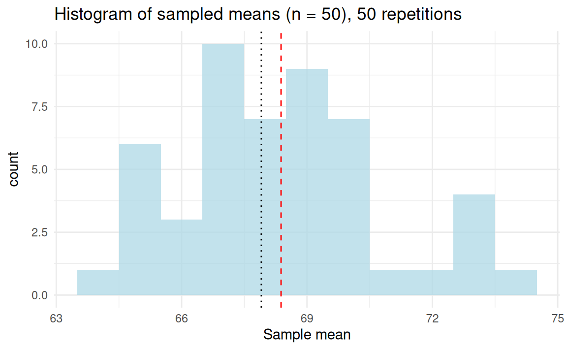
Taking samples from the YRBSS data

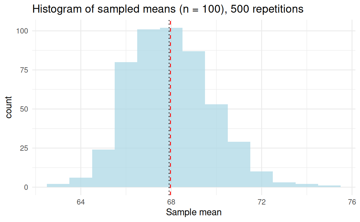
The estimator $\bar{X}$ is a random variable—randomness from sampling.

The sample mean as a random variable

The statistic $\bar{X}$ is a random variable for which $\bar{X} \sim N (μ, σ_{\bar{X}}^{2})$

The sampling distribution of $\bar{X}$ is centered around $μ$ because $\bar{X} \to μ$ (consistency, strong law of large numbers).
The variability of $\bar{X}$ becomes smaller with larger sample size, $n$ .

Any sample statistic is a random variable since each sample drawn from the population ought to be different.

When the data have not yet been observed, the statistic, like the corresponding RV, is a function of the same random elements.

The standard error of $\bar{X}$

If $\bar{X}$ could be observed through repeated sampling, its standard deviation would be ${SE}_{\bar{X}} = \frac{σ_{X}}{\sqrt{n}}$ (n.b., ${SE}_{\bar{X}} = \sqrt{σ_{\bar{X}}^{2}}$ )

The variability of a sample mean decreases as sample size increases: ${SE}_{\bar{X}}$ characterizes that behavior more precisely.

Typically, $σ_{X}$ is unknown and estimated by $s_{X}$ .
The term $\frac{s_{X}}{\sqrt{n}}$ is called the standard error of $\bar{X}$ .

Leveraging variability: Confidence intervals

A confidence interval gives a plausible range of values for the population parameter, coupling an estimate and a margin of error:

Confidence intervals: Definition and construction

A confidence interval with coverage rate $1 - α$ for a population mean $μ$ is any random interval ${CI}_{(1 - α)} (μ)$ such that $P [μ \in {CI}_{(1 - α)} (μ)] \geq 1 - α$ . A common form is $\bar{x} \pm m \to (\bar{x} - m, \bar{x} + m),$ where the margin of error, $m$ , draws on the sampling variability of $\bar{X}$ .

Since $\sqrt{n} (\bar{X} - μ) \to_{d} N (0, σ^{2})$ , the margin of error may be based on the properties (e.g., quantiles) of the normal distribution.

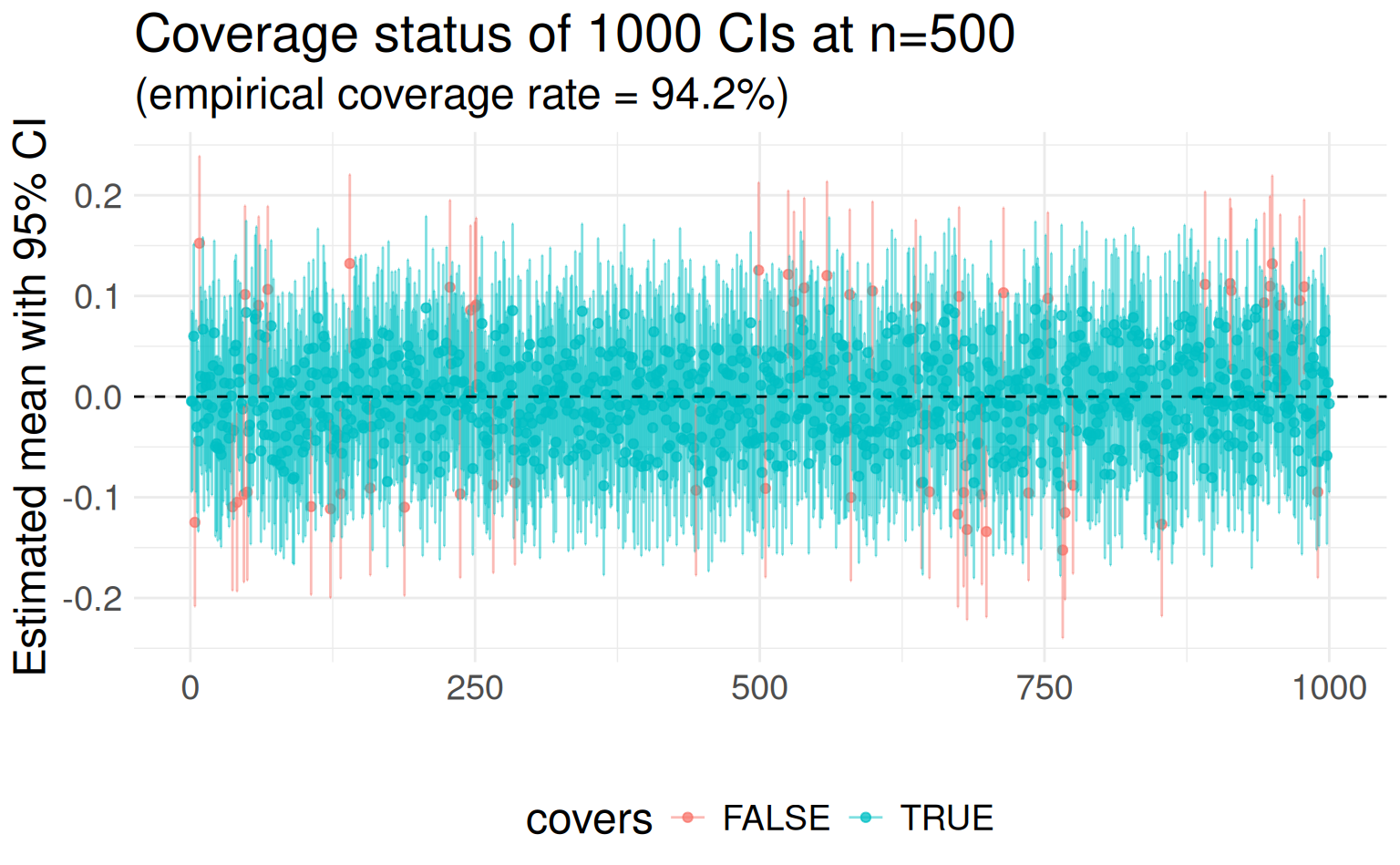
Confidence intervals: The fine print…

The confidence level may also be called the confidence coefficient. Confidence intervals have a nuanced interpretation:

The method for computing a 95% confidence interval produces a random interval that—on average—contains the true (target) population parameter 95 times out of 100.
5 out of 100 will be incorrect, but, of course, a data analyst (or reader of your paper!) cannot know whether a particular interval contains the true population parameter.
The data used to calculate the confidence interval are from a random sample taken from a well-defined target population.

Confidence intervals: Proof by picture

Asymptotic $1 - α$ (100)% CI

Random interval ${CI}_{(1 - α)} (μ)$ is a $(1 - α)$ (100)% CI if $lim_{n \to \infty} P [μ \in {CI}_{(1 - α)} (μ)] \geq 1 - α$

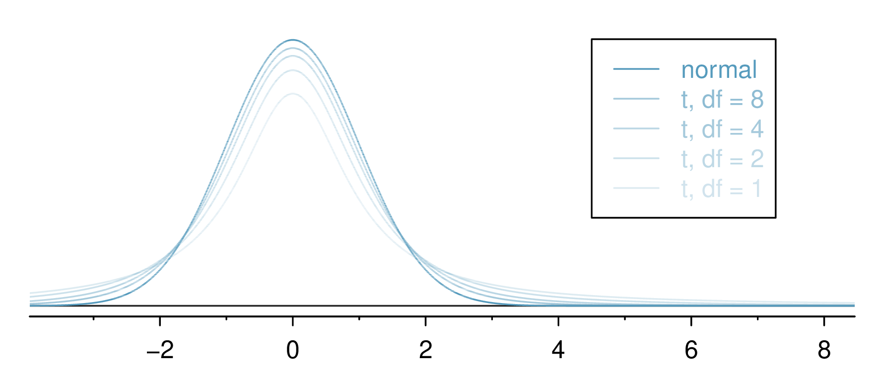
The $t$ Distribution

The $t$ distribution¹ is symmetric, bell-shaped, and centered at zero; it is like a standard normal distribution $N (0, 1)$ , almost…

It has an additional parameter–degrees of freedom ( $d f$ or $ν$ ).

Degrees of freedom ( $d f$ ) equals $ν = n - 1$ .
The $t$ distribution’s tails are thicker than those of a normal.
When $d f$ is “large” ( $d f \geq 30$ ), the $t$ and $N (0, 1)$ distributions are virtually identical (technically, only when $ν \to \infty$ ).

The $t$ Distribution…

A ( $1 - α$ )(100)% confidence interval

A ( $1 - α$ )(100)% confidence interval (CI) for a population mean $μ$ based on a single sample with mean $\bar{x}$ is

$\bar{x} \pm t^{⋆} \times \frac{s}{\sqrt{n}} \to (\bar{x} - t^{⋆} \frac{s}{\sqrt{n}}, \bar{x} + t^{⋆} \frac{s}{\sqrt{n}}),$ where $t^{⋆}$ is the quantile of a $t$ distribution (with $ν = n - 1$ df) for which there is $1 - \frac{α}{2}$ area to its left.

For a 95% CI, find $t^{⋆}$ with 0.975 area to its left (or, equivalently, 0.025 area to its right).

Calculating the critical $t$ -value, $t^{⋆}$

The R function qt(p, df) finds the quantile of a $t$ distribution with df degrees of freedom that has area $p = P (T \leq t)$ to its left.

$t^{⋆}$ for a 95% confidence interval where $n = 10$ is 2.262.
```
qt(0.975, df = 9)
```
```
[1] 2.262157
```

Just let R do the work for you…95% CI from t.test():

set.seed(02115)
n_sample <- 10
sampled_rows <- sample(1:nrow(yrbss), n_sample)
t.test(yrbss$weight[sampled_rows])$conf.int

[1] 61.12566 77.87656
attr(,"conf.level")
[1] 0.95

Inference: Testing a hypothesis

Question: Do Americans tend to be overweight?

Body mass index (BMI) is a scale used to assess weight status, adjusting for height.
The CDC’s National Health and Nutrition Examination Survey (NHANES) assesses health and nutritional status of adults, children in the US.

WHO BMI standards (Vu and Harrington 2020, Table 4.12)
Category	BMI range
Underweight	$< 18.50$
Healthy weight	18.5-24.99
Overweight	$\geq 25$
Obese	$\geq 30$

The NHANES sample

nhanes.samp.adult (from the oibiostat R package):
- random sample from participants in NHANES in the US
- contains data on participants who were aged 21 or older at time of response

Can we use a 95% confidence interval? Yes!

Confidence interval suggests that population average BMI is well outside the range defined as healthy (BMI of 18.5-24.99):

t.test(nhanes.samp.adult$BMI, conf.level=0.95)$conf.int

[1] 27.81388 30.38524
attr(,"conf.level")
[1] 0.95

If a ( $1 - α$ )(100)% confidence interval for a population mean does not contain a hypothesized value $μ_{0}$ , then:

the observed data contradict the null hypothesis $H_{0} : μ = μ_{0}$ (at a given significance level $α$ , e.g., $α = 0.05$ )
the implied two-sided alternative hypothesis is $H_{A} : μ \neq μ_{0}$

Null and alternative hypotheses

The null hypothesis ( $H_{0}$ ) posits a distribution for the population reflecting no change from the past, e.g., $H_{0} : μ = μ_{0}$ .
The alternative hypothesis ( $H_{A}$ ) claims a “real” difference exists between the distribution of the observed data (a sample) and the distribution implied by the null hypothesis.¹
Since $H_{A}$ is an alternative claim, it is often represented by a range of possible parameter values, e.g., $H_{A} : μ \neq μ_{0}$ .
A hypothesis test evaluates whether there is evidence against $H_{0}$ based on the observed data, using a test statistic.

Framing null and alternative hypotheses

For our BMI inquiry, there are a few possible choices for $H_{0}$ and $H_{A}$ . To simplify and demonstrate, let’s use

$H_{0} : μ_{BMI} = 21.7 = μ_{0}$ , the midpoint of the healthy range
$H_{A} : μ_{BMI} > 21.7$

The form of $H_{A}$ above is a one-sided alternative. One could also write a two-sided alternative, $H_{A} : μ_{BMI} \neq 21.7$ .

The choice of one- or two-sided alternative is context-dependent and should be driven by the motivating scientific question.

What’s “real”? The significance level $α$

The significance level $α$ quantifies how rare or unlikely an event must be in order to represent sufficient evidence against $H_{0}$ .

In other words, it is a bar for the degree of evidence necessary for a difference to be considered as “real” (or significant)¹ ².

In the context of decision errors, $α$ is the probability of committing a Type I error (incorrectly rejecting $H_{0}$ when it is true).

Choose (and calculate) a test statistic

The test statistic measures the discrepancy between the observed data and what would be expected if the null hypothesis were true.

When testing hypotheses about a mean, a valid test statistic is $T = \frac{\bar{X} - μ_{0}}{\frac{s}{\sqrt{n}}},$ where the test statistic $T$ follows a $t$ distribution with $ν = n - 1$ .

The devil is in the details

We will go on to talk about a few more practical versions of the $t$ -test (e.g., 2-sample $t$ -test, 1-sample $t$ -test of paired differences).

In each of these cases, some assumptions are required…

measurements being compared (e.g., BMI) are randomly (iid) sampled from a normal distribution
same unknown mean, same unknown variance (plus normality)

Justifying your assumptions is the hardest part

Given the context of your scientific problem, are these assumptions true or reasonable?

Calculate a $p$ -value…and what is it anyway?

What is the probability that we would observe a result as or more extreme than the observed sample value, if the null hypothesis is true? This probability is the $p$ -value¹.

Calculate the $p$ -value associated with the test statistic and then compare it to the pre-specified significance level $α$ .
A result is considered unusual (or statistically significant) if its associated $p$ -value is less than $α$ .

Quantifying surprise – the $S$ -value

Despite their popularity, $p$ -values are notoriously hard to interpret¹. Rafi and Greenland (2020)’s $S$ -values (“binary surprisal value”) are a cognitive tool for interpreting and understanding $p$ -values².

The surprisal value $S$ for interpreting $p$ -values

The $S$ -value is defined via $p = {(\frac{1}{2})}^{s}$ as $s = - \log_{2} (p)$ , where $p$ is a $p$ -value.

$S$ quantifies the degree of surprise associated with experiencing a similar result (as the given $p$ -value) when evaluating if a coin is fair.

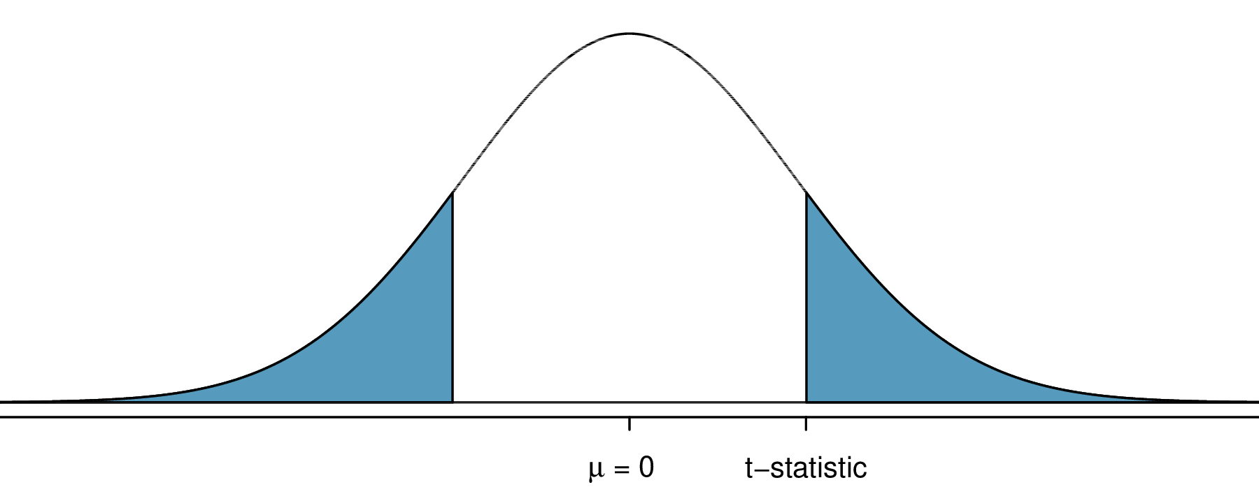
The $p$ -value for a two-sided alternative

For a two-sided alternative, $H_{A} : μ \neq μ_{0}$ , the $p$ -value of a t-test is the total area from both tails of the t distribution that are beyond the absolute value of the observed t statistic:

$p = 2 P (T \geq | t |) = P (T \leq - | t |) + P (T \geq | t |)$

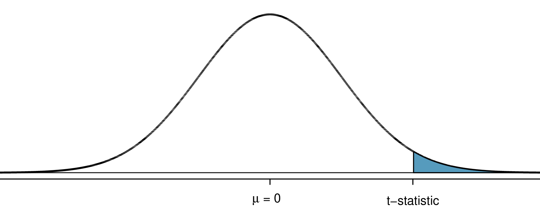
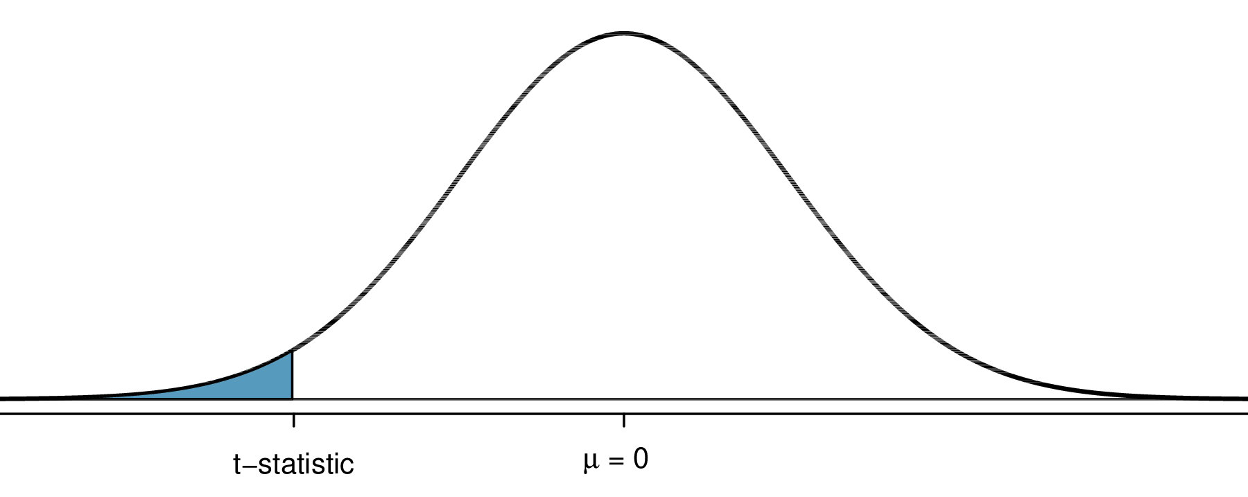
The $p$ -value for a one-sided alternative

For a one-sided alternative, the $p$ -value is the area in the tail of the t distribution that matches the direction of the alternative.

For $H_{A} : μ > μ_{0}$ : $p = P (T \geq | t |)$

For $H_{A} : μ < μ_{0}$ : $p = P (T \leq - | t |)$

The $p$ -value and drawing conclusions

The smaller the $p$ -value, the stronger the evidence against $H_{0}$ .

If the $p$ -value is as small or smaller than $α$ , we reject $H_{0}$ ; the result is statistically significant at level $α$ .
If the $p$ -value is larger than $α$ , we fail to reject¹ $H_{0}$ ; the result is not statistically significant at level $α$ —that is, the evidence we have available does not contradict $H_{0}$ .

Always state conclusions in the context of the research problem.

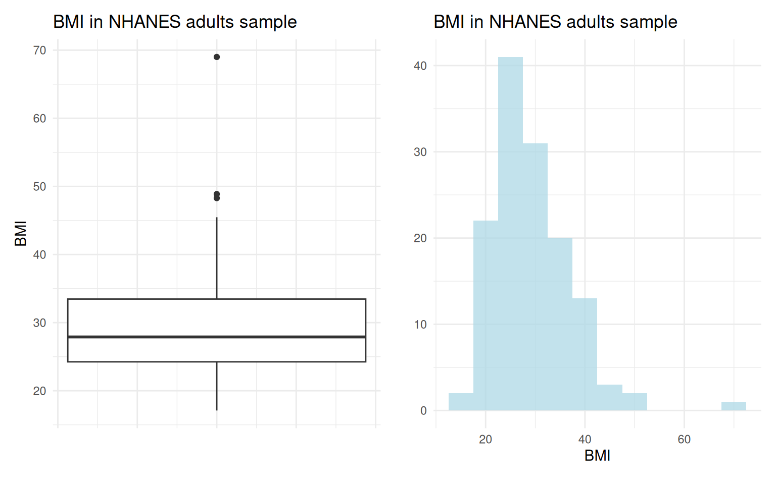
Evaluating BMI in the NHANES adult sample

Question: Do Americans tend to be overweight?

# use R as a calculator...
x_bar <- mean(nhanes.samp.adult$BMI)
mu_0 <- 21.7
s <- sd(nhanes.samp.adult$BMI)
n <- length(nhanes.samp.adult$BMI)
(t <- (x_bar - mu_0) / (s / sqrt(n)))

[1] 11.38311

pt(t, df = n - 1, lower.tail = FALSE)

[1] 1.006759e-21

# just let R do the work...
t.test(
  nhanes.samp.adult$BMI, mu = 21.7,
  alternative = "greater"
)


    One Sample t-test

data:  nhanes.samp.adult$BMI
t = 11.383, df = 134, p-value < 2.2e-16
alternative hypothesis: true mean is greater than 21.7
95 percent confidence interval:
 28.02288      Inf
sample estimates:
mean of x 
 29.09956

The Kolmogorov-Smirnov (KS) test

The KS test is a nonparametric test that evaluates the equality of two distributions (n.b., different from testing mean differences).

The empirical cumulative distribution function (eCDF) is $F_{n} (x) = \frac{1}{n} \sum_{i = 1}^{n} I_{(- \infty, x)} (X_{i}) = \frac{# elements \leq x}{n}$

The KS test uses as its test statistic $D_{n} = {sup}_{x} | F_{n} (x) - F (x) |$ ¹, where $F (x)$ is a theoretical (i.e., assumed) CDF.

Using the KS test: Is BMI normally distributed?

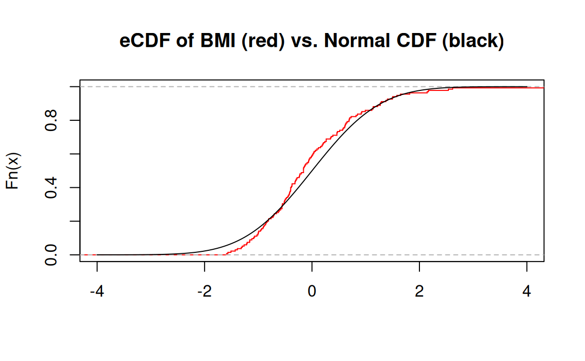
Applying the KS test evaluates evidence against $H_{0}$ of BMI (in NHANES population) arising from a normal distribution:


    Asymptotic one-sample Kolmogorov-Smirnov test

data:  bmi_zstd
D = 0.09895, p-value = 0.1422
alternative hypothesis: two-sided

References

Cole, Stephen R, Jessie K Edwards, and Sander Greenland. 2021. “Surprise!” American Journal of Epidemiology 190 (2): 191–93. https://doi.org/10.1093/aje/kwaa136.

Fisher, Ronald Aylmer. 1926. “The Arrangement of Field Experiments.” Journal of the Ministry of Agriculture of Great Britain 33: 503–13.

Freedman, David A, Robert Pisani, and Roger Purves. 2007. Statistics. W. W. Norton & Company.

Mendenhall, William, Robert J Beaver, and Barbara M Beaver. 2012. Introduction to Probability and Statistics. Cengage Learning.

Rafi, Zad, and Sander Greenland. 2020. “Semantic and Cognitive Tools to Aid Statistical Science: Replace Confidence and Significance by Compatibility and Surprise.” BMC Medical Research Methodology 20: 244. https://doi.org/10.1186/s12874-020-01105-9.

Senn, Stephen. 2022. Dicing with Death: Living by Data. Cambridge University Press. https://doi.org/10.1017/9781009000185.

Student. 1908. “The Probable Error of a Mean.” Biometrika 6 (1): 1–25. https://doi.org/10.1093/biomet/6.1.1.

Vu, Julie, and David Harrington. 2020. Introductory Statistics for the Life and Biomedical Sciences. OpenIntro. https://openintro.org/book/biostat.