Elements of Statistical Inference, Part II

Nima Hejazi

nhejazi@hsph.harvard.edu

Harvard Biostatistics

July 8, 2025

- The project is out-of-sync -- use `renv::status()` for details.

Comparing two population parameters

Two-sample data can be paired or unpaired (independent).

• Paired measurements for each “participant” or study unit

  • each unit can be matched to another unit in the data
  • e.g., “enriched” vs. “normal” environments for pairs of rats, with pairs taken from the same litter

• Two independent sets of measurements

  • observations cannot be matched on a one-to-one basis
  • e.g., rats from several distinct litters observed in either “enriched” or “normal” environments

Nature of the data dictates testing procedure: two-sample test for paired data or two-sample test for independent group data.

Example: Menstruation’s effect on energy intake

Does the dietary (energy) intake of women differ pre- versus post-menstruation (across 10 days)? (Table 9.3 of Altman 1990)

A study was conducted to assess the effect of menstruation on energy intake.

• \(n=11\) women’s dietary (energy) intake was measured pre- and post- (10 days)
• Investigators recorded energy intake for each of the women (in kJ)

pre	post
5260	3910
5470	4220
5640	3885
6180	5160
6390	5645
6515	4680

The paired \(t\)-test

The energy intake measurements are paired within a given study unit (each of the women)—use this structure to advantage, i.e., exploit homogeneity.

For each woman \(i\), we have measurements \(x_{i, \text{pre}}\) and \(x_{i, \text{post}}\).

• Define the measurement difference: \(d_i = x_{i, \text{pre}} - x_{i, \text{post}}\)

  • \(x_{i, \text{pre}}\) is the energy intake pre-menstruation for woman \(i\)
  • \(x_{i, \text{post}}\) is the energy intake post-menstruation for woman \(i\)

• Base inference on \(\overline{d}\), sample mean of the \(d_i\), that is \(\overline{d} = \frac{1}{n} \sum_{i=1}^n d_i\)

The paired \(t\)-test

Let \(\Delta\) be the population mean of the difference in energy intake for 10-day intervals pre- and post-menstruation for the population of women from which this random sample (of \(n=11\)) was taken.

The null and alternative hypotheses are

• \(H_0: \Delta= 0\), no difference in energy intake pre- vs. post-
  • i.e., no effect of menstruation on subsequent energy intake
• \(H_A: \Delta \neq 0\), there is a difference in energy intake pre- vs. post-
  • i.e., menstruation does have an effect on energy intake

The paired \(t\)-test and confidence interval

The test statistic for the paired \(t\)-test is

\(t\)-test and confidence interval for paired data

\[ t = \dfrac{\overline{d} - \Delta_{H_0}}{\dfrac{s_d}{\sqrt{n}}} \quad \quad \quad \text{CI}(\Delta) = \overline{d} \pm \left( t^{\star} \times \dfrac{s_d}{\sqrt{n}} \right) \] where \(\overline{d} = \frac{1}{n} \sum_{i=1}^n d_i\) is the mean of the paired differences \(d_i\), \(s_d\) is the sample standard deviation of the \(d_i\), and \(n\) is the number of differences (i.e., number of pairs).

A paired \(t\)-test is just a one-sample test of the differences \(d_i\); the \(p\)-value may be calculated from a \(t\) distribution with \(df = n - 1\). In the above, recall that \(\dfrac{s_d}{\sqrt{n}}\) is the standard error of the mean of the differences, \(\overline{d}\).

Letting R do the work

Paired \(t\)-test

# two-sample syntax
t.test(
 intake$pre, intake$post,
 paired = TRUE,
 alternative = "two.sided"
)

    Paired t-test

data:  intake$pre and intake$post
t = 11.941, df = 10, p-value = 3.059e-07
alternative hypothesis: true mean difference is not equal to 0
95 percent confidence interval:
 1074.072 1566.838
sample estimates:
mean difference 
       1320.455 

Differences \(t\)-test

# one-sample syntax
t.test(
 intake[, pre - post],
 mu = 0, paired = FALSE,
 alternative = "two.sided"
)

    One Sample t-test

data:  intake[, pre - post]
t = 11.941, df = 10, p-value = 3.059e-07
alternative hypothesis: true mean is not equal to 0
95 percent confidence interval:
 1074.072 1566.838
sample estimates:
mean of x 
 1320.455 

Independent \(t\)-test

# two-sample syntax
t.test(
 intake$pre, intake$post,
 mu = 0,  paired = FALSE,
 alternative = "two.sided"
)

    Welch Two Sample t-test

data:  intake$pre and intake$post
t = 2.6242, df = 19.92, p-value = 0.01629
alternative hypothesis: true difference in means is not equal to 0
95 percent confidence interval:
  270.5633 2370.3458
sample estimates:
mean of x mean of y 
 6753.636  5433.182 

Assumptions for paired \(t\)-test

Like the one-sample version, paired \(t\)-test requires assumptions:

• Differences arise as iid samples from \(\text{N}(0, \sigma^2_{\Delta})\), that is, from a normal distribution…
  • …assumed to have zero mean (under \(H_0\) of no difference¹)
  • …assumed to have unknown variance (i.e., \(\sigma^2_{\Delta}\))
• Additionally requirements include independence of pairs and non-interference (that is, one pair cannot affect another)
• For example, difference of pre- and post-menstruation energy intake assumed to be normally distributed

1. The assumed \(H_0\) is a weak null hypothesis of no average effect (or association)

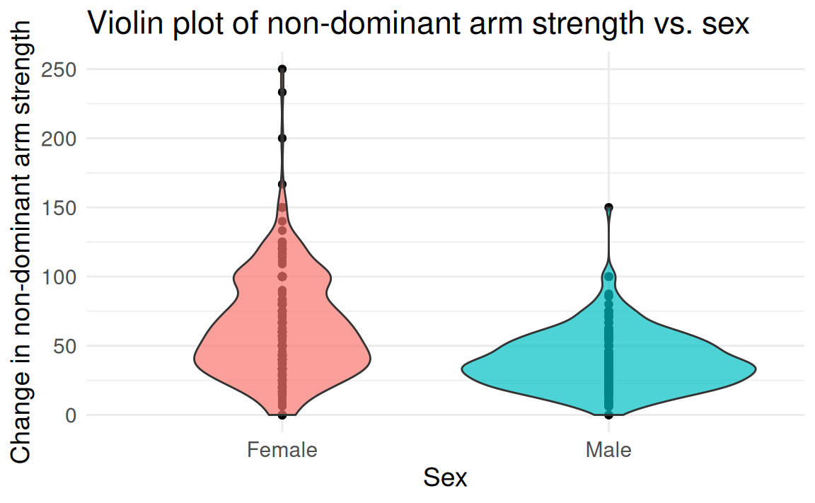
FAMuSS: Comparing arm strength by sex

Question: Does change in non-dominant arm strength (ndrm.ch) after resistance training differ between men and women?

first 6 observations from the famuss dataset

sex	age	height	weight	actn3.r577x	ndrm.ch
Female	27	65.0	199	CC	40
Male	36	71.7	189	CT	25
Female	24	65.0	134	CT	40
Female	40	68.0	171	CT	125
Female	32	61.0	118	CC	40
Female	24	62.2	120	CT	75

famuss dataset from Vu and Harrington (2020)

The two-group (independent) \(t\)-test

Framing the question — the null and alternative hypotheses are

• \(H_0: \mu_{\text{F}} = \mu_{\text{M}}\), population mean change in arm strength for women same as population mean change for men
  • Equivalently, let \(\Delta = \mu_{\text{F}} - \mu_{\text{M}}\), then \(H_0: \Delta = 0\)
• \(H_A: \mu_{\text{F}} \neq \mu_{\text{M}}\), population mean change in arm strength for women differs from population mean change for men

Hypotheses may generically be written in terms of \(\mu_A\) and \(\mu_B\).

• The parameter of interest is \(\Delta_{\mu} = \mu_A - \mu_B\).
• The point estimate is \(d_{\overline{x}} = \overline{x}_A - \overline{x}_B\).

The two-group (independent) \(t\)-test

The test statistic for the two-group (independent) \(t\)-test is

Two-group (independent) \(t\)-test

\[t = \dfrac{(\bar{x}_A - \bar{x}_B) - (\mu_A - \mu_B)} {\sqrt{\dfrac{s_A^2}{n_A} + \dfrac{s_B^2}{n_B}}} = \dfrac{d_{\overline{x}} - \Delta_{\mu}}{\sqrt{\dfrac{s_A^2}{n_A} + \dfrac{s_B^2}{n_B}}},\] where \(\sqrt{\dfrac{s_A^2}{n_A} + \dfrac{s_B^2}{n_B}}\) is an estimate of the standard errors of the two group means.

The two-sample \(t\)-test compares between-group differences; the \(p\)-value may be calculated from the \(t\) distribution, but the \(df\) differ.

\(df\) for two-group (independent) \(t\)-test

A conservative approximation is \(df = \text{min}(n_A - 1, n_B - 1)\)

The Welch-Satterthwaite approximation¹ (used by R): \[df = \dfrac{\left[s_A^2 / n_A + s_B^2 / n_B \right]^2} {\left[\dfrac{(s_A^2/n_A)^2}{(n_A - 1)} + \dfrac{(s_B^2/n_B)^2}{(n_B - 1)}\right]}\]

Alternative is to use Student’s version \(df = n_A + n_B - 2\), under a (strong!) assumption of equal variances of the two groups \(A\) and \(B\)

1. This approximates effective degrees of freedom, without assuming equality of variances

Confidence intervals for the two-group (independent) difference-in-means

A \((1-\alpha)\)(100)% confidence interval (CI) for the difference in the two population means \(\Delta_{\mu} = \mu_A - \mu_B\) is of the form

\[\text{CI}(\mu_A - \mu_B) = (\overline{x}_A - \overline{x}_B) \pm \left(t^{\star} \times \sqrt{\frac{s_A^2}{n_A} + \frac{s_B^2}{n_B}} \right),\] where \(t^{\star}\) is the critical point (i.e., quantile) on a \(t\) distribution (with same \(df\) as for corresponding \(t\)-test) and area \(\dfrac{\alpha}{2}\) in either tail.

Letting R do the work

    Welch Two Sample t-test

data:  famuss$ndrm.ch[female] and famuss$ndrm.ch[male]
t = 10.073, df = 574.01, p-value < 2.2e-16
alternative hypothesis: true difference in means is not equal to 0
95 percent confidence interval:
 19.07240 28.31175
sample estimates:
mean of x mean of y 
 62.92720  39.23512 

uses \(\sqrt{\dfrac{s_A^2}{n_A} + \dfrac{s_B^2}{n_B}}\)

    Two Sample t-test

data:  famuss$ndrm.ch[female] and famuss$ndrm.ch[male]
t = 9.1425, df = 593, p-value < 2.2e-16
alternative hypothesis: true difference in means is not equal to 0
95 percent confidence interval:
 18.60259 28.78155
sample estimates:
mean of x mean of y 
 62.92720  39.23512 

uses¹ \(s_{\text{pooled}} \sqrt{\dfrac{1}{n_A} + \dfrac{1}{n_B}}\)

1. \(s_{\text{pooled}} = \sqrt{\{s_A^2(n_A - 1) + s_B^2(n_B - 1)\} / \{n_A + n_B - 2\}}\) with \(df = n_A + n_B - 2\)

Assumptions for two-group (independent) \(t\)-test

• Observations arise as iid samples from \(\text{N}(\mu, \sigma^2)\), that is, from a normal distribution common between the two populations…
  • …assumed to have same population mean (under \(H_0\)¹)
  • …assumed to have same unknown variance² (i.e., \(\sigma^2\))
• Additional requirements include independence of observations and non-interference (one observation cannot affect another)
• For example, change in non-dominant arm strength for men and women is assumed to follow \(\text{N}(\mu, \sigma^2)\) with a common variance \(\sigma^2\), or \(\text{N}(\mu, \sigma^2_M)\) and \(\text{N}(\mu, \sigma^2_F)\) for males, females

1. The assumed \(H_0\) is a weak null hypothesis of no average effect (or association)

2. This can be relaxed, though the relevant \(df\) becomes more complicated

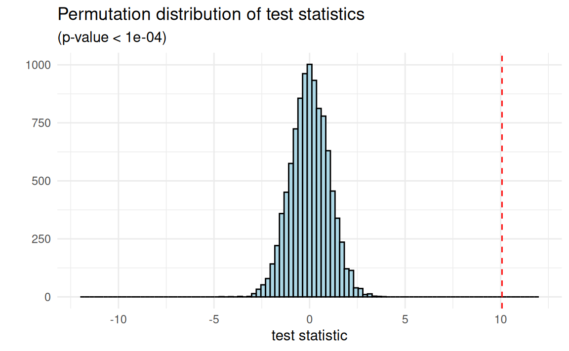
Permutation-based hypothesis testing

Permutation testing¹ is a nonparametric framework for inference

• aim is to limit assumptions about the underlying populations, instead using structure that can be induced by design
• method: construct the null distribution of a test statistic via (artificial) randomization, as if assignment² was controlled

Permutation/randomization inference evaluates evidence against a different null hypothesis (\(H_0: X_{i,A} = X_{i,B} \,\, \forall \,\, i = 1, \ldots, n\))

1. The assumed \(H_0\) is a sharp null hypothesis of no individual effect (or association)

2. Here, we envisage exchangeability of the characteristic that is being evaluated

Assumptions for permutational \(t\)-test

• Unlike the paired or two-group \(t\)-test discussed so far,
  • …there is no need to assume a specific distributional form for how the data—observations or paired differences—arise
  • …non-interference issues (units cannot affect each other) are resolved by the construction of the null hypothesis
• So…what do we need then?
  • Groups (or differences) are exchangeable (under \(H_0\))—no relationship between assignment and outcome
  • Randomization (of assignment) is performed fairly

The permutational \(t\)-test in action

    Exact Two-Sample Fisher-Pitman Permutation Test

data:  ndrm.ch by sex (Female, Male)
Z = 8.5664, p-value < 2.2e-16
alternative hypothesis: true mu is not equal to 0

Exact: How many ways to choose \(n=\) 242 males from \(n=\) 595 individuals? 1.294158^{173}!

    Approximative Two-Sample Fisher-Pitman Permutation Test

data:  ndrm.ch by sex (Female, Male)
Z = 8.5664, p-value < 1e-04
alternative hypothesis: true mu is not equal to 0

Approximate: What about 10000? Is that enough?

Null hypotheses: The weak and the sharp

Data on \(n\) units, measured as \(X_1, \ldots, X_n\), under two conditions \(A\) and \(B\), e.g., \(n = 1000\) patients assigned treatment \(A\) or placebo \(B\)

Weak null: averages

\(H_0: \mu_A = \mu_B\)

\(H_A: \mu_A \neq \mu_B\)

Is there no effect on average?

Sharp (strong) null: individuals

\(H_0: X_{i, A} = X_{i, B} \,\, \forall \,\, i\)

\(H_A: X_{i, A} \neq X_{i, B} \,\, \text{for some} \,\, i\)

Is there no effect for everyone?

The sharp null implies the weak null—no effect at all, no effect on average too.

FAMuSS: Comparing arm strength by genotype

Going beyond two-group comparisons

Is change in non-dominant arm strength after resistance training associated with genotype?

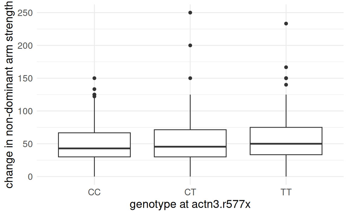
• \(H_0: \mu_{CC} = \mu_{CT} = \mu_{TT}\): mean change in arm strength is equal across the three genotypes
• \(H_A: \mu_{CC} \neq_? \mu_{CT} \neq_? \mu_{TT}\): at least one genotype has mean change in arm strength differing from others

Analysis of Variance (ANOVA)

Suppose we are interested in comparing means across more than two groups. Why not conduct several two-sample \(t\)-tests?

• If there are \(k\) groups, then \({k \choose 2} = \frac{k(k-1)}{2}\) \(t\)-tests are needed.
• Conducting multiple tests on the same data increases the overall rate of Type I error, necessitating a multiplicity correction.

ANOVA: Assesses equality of means across many groups:

• \(H_0\): means equal across all groups (\(\mu_A = \mu_B = \ldots = \mu_k\))
• \(H_A\): at least one mean differs from others (i.e., not all equal)

ANOVA: Are the groups all the same?

Under \(H_0\), there is no real difference between the groups—so any observed variation in group means must be due to chance alone.

• Think of all observations as belonging to a single, large group.
• Variability between group means \(\approx\) Variability within groups

ANOVA exploits differences in means from an overall mean and within-group variation to evaluate equality of a few group means.

ANOVA: Are the groups all the same?

Is the variability in the sample means large enough that it seems unlikely to be due to chance alone?

Compare two quantities:

• Variability between groups (\(MS_{\text{Groups}}\)¹): how different are the group means from each other, i.e., relative to the overall mean?
• Variability within groups (\(MS_{\text{Error}}\)²): how variable are the data within each group?

1. \(MS_{\text{Groups}}\) denotes mean square between groups

2. \(MS_{\text{Error}}\) denotes mean square error (not mean squared error)

ANOVA: The \(F\)-statistic

The \(F\)-test for ANOVA

ANOVA measures discrepancies via the F-statistic, which follows an \(F\) distribution: \[ F = \frac{\text{variance between groups}}{\text{variance within groups}} = \frac{MS_{\text{Groups}}}{MS_{\text{Error}}} \]

• \(F \approx 1\) when the population means are equal.
• \(F > 1\), larger values, stronger evidence against \(H_0\).
• The \(F\)-statistic follows an \(F\) distribution, with two degrees of freedom, \(df_1 = n_{groups} - 1\), \(df_2 = n_{obs} - n_{groups}\).
• \(p\)-value: Probability \(F\) is larger than the \(F\)-statistic under \(H_0\).

Assumptions for ANOVA

Just like the \(t\)-test, ANOVA requires assumptions about the data

• Observations are independent within and across groups
• Data within each group arise from a normal distribution
• Variability across the groups is about equal

When these assumptions are violated, hard to know whether \(H_0\) being rejected is due to evidence or failure of the assumptions…

As with the \(t\)-test, a permutational \(F\)-test can be formulated.

Pairwise comparisons

If the \(F\)-test indicates sufficient evidence of inequality of the group means, pairwise comparisons to identify the group may follow.

Pairwise comparisons may use the two-group (independent) \(t\)-test:

• To maintain overall Type I error rate at \(\alpha\), each comparison should be conducted at at an adjusted significance level, \(\alpha^\star\).
• The Bonferroni correction¹ is one method for adjusting \(\alpha\), using \(\alpha^{\star} = \alpha / K\), where \(K = {k \choose 2} = \frac{k(k-1)}{2}\) for \(k\) groups.
• Note: The Bonferroni correction is conservative (i.e., stringent), and assumes all tests are independent.

1. The Bonferroni correction just divides \(\alpha\) by the number of tests (e.g., \(K\)) to arrive at \(\alpha^{\star}\)

Letting R do the work

# use summary(aov())
summary(aov(famuss$ndrm.ch ~ famuss$actn3.r577x))

                    Df Sum Sq Mean Sq F value Pr(>F)  
famuss$actn3.r577x   2   7043    3522   3.231 0.0402 *
Residuals          592 645293    1090                 
---
Signif. codes:  0 '***' 0.001 '**' 0.01 '*' 0.05 '.' 0.1 ' ' 1

Conclusion: \(p < \alpha\), sufficient evidence to reject \(H_0\) in favor of \(H_A\)—so at least one group differs in mean from the others.

But which group(s) is (are) the source of the difference? 🧐

Controlling Type I error rate

If the \(F\)-test indicates sufficient evidence of inequality of the group means, pairwise comparisons (\(t\)-tests¹) may identify those groups.

• Each test should be conducted at the \(\alpha^\star\) significance level so that the overall Type I error rate remains at \(\alpha\).
• These \(t\)-tests are conducted under the assumption that the between-group variance is equal, using the pooled SD estimate.
• We will use pairwise.t.test() to perform these post hoc two-sample t-tests.

1. \(t\)-tests conducted in this way are typically referred to as post hoc tests.

Controlling Type I error rate

Pairwise comparisons using two-sample \(t\)-tests (CC to CT, CC to TT, CT to TT) can now be done if the Type I error rate is controlled.

• Apply the Bonferroni correction.
• In this setting, \(\alpha^{\star} = 0.05/3 = 0.0167\).

Examine each of the three two-sample \(t\)-tests, evaluating evidence for group mean differences at the more stringent level of \(\alpha^{\star}\).

Letting R do the work

Only CC versus TT resulted in a \(p\)-value less than \(\alpha^{\star} = 0.0167\).

• Mean strength change in non-dominant arm for individuals with genotype CT is not distinguishable from strength change for those with CC and TT.
• However, evidence at \(\alpha = 0.05\) level that mean strength change for individuals of genotype CC and TT are different.

\(p\)-values on original scale (compare to \(\alpha^{\star}\))

pairwise.t.test(
  famuss$ndrm.ch, famuss$actn3.r577x, p.adj = "none"
)

    Pairwise comparisons using t tests with pooled SD 

data:  famuss$ndrm.ch and famuss$actn3.r577x 

   CC    CT   
CT 0.179 -    
TT 0.011 0.144

P value adjustment method: none 

\(p\)-values on corrected scale (compare to \(\alpha\))

pairwise.t.test(
  famuss$ndrm.ch, famuss$actn3.r577x, p.adj = "bonf"
)

    Pairwise comparisons using t tests with pooled SD 

data:  famuss$ndrm.ch and famuss$actn3.r577x 

   CC    CT   
CT 0.537 -    
TT 0.034 0.433

P value adjustment method: bonferroni 

Type I error rate for a single test

Hypothesis testing was intended for controlled experiments or for studies with only a few comparisons (e.g., ANOVA).

Type I errors (rejecting \(H_0\) when \(H_0\) true) occur with probability \(\alpha\).

• Type I error rate is controlled by rejecting only when the \(p\)-value of a test is smaller than \(\alpha\) (where \(\alpha\) is typically kept low).
• With a single two-group comparison at \(\alpha = 0.05\), 5% chance of incorrectly identifying an association where none exists.

And what about many tests?

Multiple testing–compounding error

What happens to Type I error when making several comparisons? When conducting many tests, many chances to make a mistake.

• The significance level (\(\alpha\)) used in each test controls the error rate for that test only.
• Experiment-wise error rate: the chance of at least one test incorrectly rejecting \(H_0\) when all of the null hypotheses are true (the “global null”).
• Controlling the experiment-wise error¹ rate is just one approach for controlling the Type I error.

1. Experiment-wise error rate is closely related to family-wise error rate (FWER) and distinct from the false discovery rate (FDR) (Benjamini and Hochberg 1995)

Probability of experiment-wise error

A scientist is using two \(t\)-tests to examine a possible association of each of two genes with a disease type. Assume the tests are independent and each are conducted at level \(\alpha = 0.05\).

• \(A\): event of making a Type I error on the first test,
• \(B\): event of making a Type I error on the second test,
• Control \(\mathbb{P}(A) = \mathbb{P}(B) = 0.05\) for overall \(\alpha = 0.05\).

Example of compounding of Type I error

Probability of making at least one error is equal to the complement of the event that a Type I error is not made with either test. \[1 - [\mathbb{P}(A^C) \mathbb{P}(B^C) ] = 1 - (1 - 0.05)^2 = 0.0975\]

Probability of experiment-wise error…

10 tests… \(\text{experiment-wise error }= 1 - (1 - 0.05)^{10} = 0.401\)

25 tests… \(\text{experiment-wise error }= 1 - (1 - 0.05)^{25} = 0.723\)

100 tests… \(\text{experiment-wise error }= 1 - (1 - 0.05)^{100} = 0.994\)

With 100 independent tests: 99.4% chance an investigator will make at least one Type I error!

Advanced melanoma

Advanced melanoma is an aggressive form of skin cancer that until recently was almost uniformly fatal.

Research is being conducted on therapies that might be able to trigger immune responses to the cancer that then cause the melanoma to stop progressing or disappear entirely.

In a study where 52 patients were treated concurrently with 2 new therapies, nivolumab and ipilimumab, 21 had immune responses.¹

1. Wolchok et al. (2013)

Advanced melanoma

Some research questions that can be addressed with inference…

• What is the population probability of immune response following concurrent therapy with nivolumab and ipilimumab?
• What is a 95% confidence interval for the population probability of immune response following concurrent therapy with nivolumab and ipilimumab?
• In prior studies, the proportion of patients responding to one of these agents was 30% or less. Do these data suggest a better (>30%) probability of response to the concurrent therapy?

Inference for binomial proportions

In this study of melanoma, experiencing an immune response to the concurrent therapy is a binary event (i.e., binomial data).

Suppose \(X \sim \text{Bin}(n, p)\) is a binomial RV with parameters \(n\), the number of trials, and \(p\), the probability of success.

• Goal: Inference about population parameter \(p\), the probability of success in the population¹.
• \(\hat{p} = x/n\) is the point estimate of \(p\) from the observed sample, where \(x\) is the observed number of successes.

1. For example, \(p\) would be experiencing immune response after concurrent therapy for the population of patients with advanced melanoma in Wolchok et al. (2013)’s study.

Assumptions for using the normal distribution

The sampling distribution of \(\hat{p}\) is approximately normal¹ when

1. The sample observations are independent, and
2. At least 10 successes and 10 failures are expected in the sample: \(np \geq 10\) and \(n(1-p) \geq 10\).²

Under these conditions, \(\hat{p}\) is approximately normally distributed with mean \(p\) and standard error \(\sqrt{\frac{p(1-p)}{n}}\), estimated as \(\sqrt{\frac{\hat{p}(1-\hat{p})}{n}}\).

1. Inference for \(p\) can be made using the normal approximation to the binomial, or directly using the binomial distribution.

2. This is commonly referred to as the “success-failure condition.” Why do we need it?

Inference with the normal approximation

For CIs, use \(\hat{p}\) instead of \(p\).

An approximate two-sided \((1 - \alpha)\)(100)% confidence interval for \(p\) is given by \[\hat{p} \pm Z_{1-\alpha/2} \sqrt{\dfrac{\hat{p}(1 - \hat{p})}{n}}\]

prop.test(x = 21, n = 52, conf.level = 0.95)$conf.int

[1] 0.2731269 0.5487141
attr(,"conf.level")
[1] 0.95

In hypothesis testing: \(p_0\) for \(p\).

Test statistic \(z\) for null \(H_0: p = p_0\) is \[z = \dfrac{\hat{p} - p_0}{\sqrt{\dfrac{p_0(1 - p_0)}{n}}}\]

prop.test(
  x = 21, n = 52, p = 0.30, alternative = "greater"
)

    1-sample proportions test with continuity correction

data:  21 out of 52, null probability 0.3
X-squared = 2.1987, df = 1, p-value = 0.06906
alternative hypothesis: true p is greater than 0.3
95 percent confidence interval:
 0.2906582 1.0000000
sample estimates:
        p 
0.4038462 

Exact inference for binomial data

An exact procedure does not reply upon a limit approximation.¹

The Clopper-Pearson CI is an exact method for binomial CIs: \((\inf S_{\geq}, \sup S_{\leq})\), where \[\begin{align*} S_{\leq} &:= \{p \lvert \mathbb{P} \{\text{Bin}(n,p) \leq x\} > \alpha/2\} \\ S_{\geq} &:= \{p \lvert \mathbb{P} \{\text{Bin}(n,p) \geq x\} > \alpha/2\} \end{align*}\]

Note: While exactness is by construction, the CIs can be conservative (i.e., too large) relative to those from an approximation.

# use pbinom
pbinom(20, 52, p = 0.30, lower.tail = FALSE)

[1] 0.07167176

# use binom.test
binom.test(
  x = 21, n = 52, p = 0.30,
  alternative = "greater"
)

    Exact binomial test

data:  21 and 52
number of successes = 21, number of trials = 52, p-value = 0.07167
alternative hypothesis: true probability of success is greater than 0.3
95 percent confidence interval:
 0.2889045 1.0000000
sample estimates:
probability of success 
             0.4038462 

1. For example, the normal approximation to the binomial distribution.

Inference for difference of two proportions

The normal approximation can be applied to \(\hat{p}_A - \hat{p}_B\) if

1. The samples are independent, the observations in each sample are independent, and
2. At least 10 successes and 10 failures are expected in each sample.

The standard error of the difference in sample proportions is \[\text{SE}(p_A - p_B) = \sqrt{\dfrac{p_A(1 - p_A)}{n_A} + \dfrac{p_B(1 - p_B)}{n_B}}\]

Treating HIV\(^{+}\) infants

In resource-limited settings, single-dose nevirapine is given to HIV\(^{+}\) women during birth to prevent mother-to-child transmission of HIV.

• Exposure of the infant to nevirapine (NVP) may foster growth of resistant strains of the virus in the child.
• If the child is HIV\(^+\), should he/she be treated with nevirapine or a more expensive drug, lopinarvir (LPV)?

Here, the possible outcomes are virologic failure (virus becomes resistant) versus stable disease (virus growth is prevented).

Treating HIV\(^{+}\) infants

The results of a study comparing NVP vs. LPV in treatment of HIV-infected infants.¹ Children were randomized to receive NVP or LPV.

	NVP	LPV	Total
Virologic Failure	60	27	87
Stable Disease	87	113	200
Total	147	140	287

Is there evidence of a difference in NVP vs. LPV? How to see this?²

1. Violari et al. (2012)

2. Testing for a difference between \(p_A\) (e.g., \(p_{\text{NVP}}\)) and \(p_B\) (e.g., \(p_{\text{LPV}}\)) is equivalent to testing for association in a two-way table that has two rows and two columns.

Formulating hypotheses in a two-way table

Do data support the claim of a differential outcome by treatment?

If there is no difference in outcome by treatment, then knowing treatment provides no information about outcome, i.e., treatment assignment and outcome are independent (i.e., not associated).

• \(H_{0}\): Treatment and outcome are not associated.
• \(H_{A}\): Treatment and outcome are associated.

Question: What would we expect if no association (i.e., under \(H_0\))?

The \(\chi^2\) test of independence

Idea: How do the observed cell counts differ from those expected (under \(H_0\), i.e., as if the null hypothesis were true)? Let’s use this.

The Pearson \(\chi^2\) test of independence formulates a test statistic to quantify the magnitude of deviation of observed results from what would be expected under \(H_0\).

• Large test statistic: Stronger evidence against the null hypothesis of independence.
• Small test statistic: Weaker evidence (or lack of) against the null hypothesis of independence.

Assumptions for the \(\chi^2\) test

• Independence: Each case contributing a count to the \(2 \times 2\) table must be independent of all other cases in the \(2 \times 2\) table.
• Sample size: Each expected cell count must be greater than or equal to 10.¹ (Without enough data, what are you comparing?)

Under these assumptions, the Pearson \(\chi^2\) test statistic attains a \(\chi^2\) distribution with \(df\) tied to the number of comparisons.

1. For comparisons larger than \(2 \times 2\), some other rules of thumb may apply, e.g., “all expected counts being greater than 1” – but always consider whether you have enough data to make and justify a comparison. Better than relying upon rules of thumb, just use an exact test.

The \(\chi^2\) test statistic

The \(\chi^2\) test statistic is calculated as

The \(\chi^2\) test

\[\chi^2 = \sum_{i = 1}^r \sum_{j = 1}^c \dfrac{(O_{i, j} - E_{i, j})^2}{E_{i, j}},\] and is approximately distributed \(\chi^2\) with \(df= (r - 1)(c - 1)\), where \(r\) is the number of rows and \(c\) is the number of columns (e.g., in a \(2 \times 2\) table, \(df = 1\)).

\(O_{i,j}\) represents the observed count in row \(i\), column \(j\); \(E_{i,j}\) is its expected counterpart¹.

1. \(E_{i,j} = \{(\text{row $i$ total}) \times (\text{column $j$ total})\} / n,\) where \(n\) is the total number of observations.

Applying the \(\chi^2\) test: Treating HIV\(^+\) infants

If treatment has no effect on outcome, what would we expect?

Under the null hypothesis of independence, \[\mathbb{P}(A \cap B) = \mathbb{P}(A) \times \mathbb{P}(B) = \left(\frac{147}{287}\right) \left(\frac{87}{287}\right) \, ,\] where \(A\) = {assignment to NVP} and \(B\) = {virologic failure}. So, the expected cell count in the upper left corner of the \(2 \times 2\) table from Violari et al. (2012) would be \[\mathbb{E}(A \cap B) = n \times \mathbb{P}(A \cap B) = (287) \left(\frac{147}{287}\right) \left(\frac{87}{287}\right) = 44.56 \, .\] Thus, the scaled deviation, \((O_{i,j} - E_{i,j})^2 / E_{i,j}\), would be \((60 - 44.56)^2 / 44.56 = 5.35\)

Same logic applies for other cells…repeat three times and sum to get the \(\chi^2\) test statistic.

The \(\chi^2\) test in R

The data from Violari et al. (2012):

hiv_table

                  NVP LPV
Virologic Failure  60  27
Stable Disease     87 113

What would we expect to see under independence? (Table of \(E_{i,j}\))

                     NVP   LPV
Virologic Failure  44.56 42.44
Stable Disease    102.44 97.56

By comparing cells of these two tables (of \(O_{i,j}\) and \(E_{i,j}\)), we get the \(\chi^2\) test statistic.

R’s chisq.test() does all of this:

chisq.test(hiv_table)

    Pearson's Chi-squared test with Yates' continuity correction

data:  hiv_table
X-squared = 14.733, df = 1, p-value = 0.0001238

Conclusion: The \(\chi^2\) test finds evidence against the claimed independence of NPV and virologic failure at most reasonable significance standards (\(p\)-value < 0.001 and \(S\)-value \(= -\log_2(p) \approx\) 13).

Fisher’s exact test

R.A. Fisher proposed an exact test for contingency tables by exploiting the counts and margins, with the “reasoned basis” for the test being randomization and exchangeability (Fisher 1936).

	NVP	LPV	Total
Virologic Failure	a	b	a+b
Stable Disease	c	d	c+d
Total	a+c	b+d	n

\[\begin{align*} p &= \dfrac{{a+b \choose a}{c+d \choose c}}{{n \choose a+c}} = \dfrac{{a+b \choose b}{c+d \choose d}}{{n \choose b+d}} \\ p &= \dfrac{(a+b)! \, (c+d)! \, (a+c)! \, (b+d)!}{a! \, b! \, c! \, d! \, n!} \end{align*}\]

Here, \(p(A)\), seeing as many cases of virologic failure in the NVP group as we do see, follows exactly a hypergeometric distribution.

R’s fisher.test() does this:

fisher.test(hiv_table)

    Fisher's Exact Test for Count Data

data:  hiv_table
p-value = 0.0001037
alternative hypothesis: true odds ratio is not equal to 1
95 percent confidence interval:
 1.643280 5.127807
sample estimates:
odds ratio 
  2.875513 

Conclusion: Evidence for independence of NPV, virologic failure lacking (\(p < 0.001\)).

Lowering stakes: The lady tasting tea

“Dr. Muriel Bristol, a colleague of Fisher’s, claimed that when drinking tea she could distinguish whether milk or tea was added to the cup first (she preferred milk first). To test her claim, Fisher asked her to taste eight cups of tea, four of which had milk added first and four of which had tea added first.” Agresti (2012)

If the lady could not discriminate tea-milk ordering

	Tea first (real)	Milk first (real)	Total
Tea first (thinks)	2	2	4
Milk first (thinks)	2	2	4
Total	4	4	8

\(H_0\): Order doesn’t impact taste, so Dr. Bristol can’t tell

\(H_A\): Order does impact taste and Dr. Bristol can tell

What’s the probability of getting all four right?

If the lady could perfectly discriminate the ordering

	Tea first (real)	Milk first (real)	Total
Tea first (thinks)	4	0	4
Milk first (thinks)	0	4	4
Total	4	4	8

    Fisher's Exact Test for Count Data

data:  ladys_tea
p-value = 0.02857
alternative hypothesis: true odds ratio is not equal to 1
95 percent confidence interval:
 1.339059      Inf
sample estimates:
odds ratio 
       Inf 

The relative risk in a \(2 \times 2\) table

Relative risk (RR) measures the risk of an event occurring in one group relative to risk of same event occurring in another group.

The risk of virologic failure among the NVP group is \[\dfrac{\text{# in NVP group and had virologic failure}} {\text{total # in NVP group}} = \dfrac{60}{147} = 0.408\]

The risk of virologic failure among the LPV group is \[\dfrac{\text{# in LPV group and had virologic failure}} {\text{total # in LPV group}} = \dfrac{27}{140} = 0.193\]

RR of virologic failure for NVP vs. LPV is \(0.408/0.193 = 2.11\), so children treated with NVP are estimated to be more than twice as likely to experience virologic failure.

The odds ratio in a \(2 \times 2\) table

Odds ratio (OR) measures the odds of an event occurring in one group relative to the odds of the event occurring in another group.

The odds of virologic failure among the NVP group is \[\dfrac{\text{# in NVP group and had virologic failure}} {\text{# in NVP group and did not have virologic failure}} = \dfrac{60}{87} = 0.690\]

The odds of virologic failure among the LPV group is \[\dfrac{\text{# in LPV group and had virologic failure}} {\text{# in LPV group and did not have virologic failure}} = \dfrac{27}{113} = 0.239\]

OR of virologic failure for NVP vs. LPV is \(0.690/0.239 = 2.89\), so the odds of virologic failure when given NVP are nearly three times as large as the odds when given LPV.

Relative risk versus odds ratio

The relative risk cannot be used in studies that use outcome-dependent sampling, such as a case-control study:

• Suppose in the HIV study, researchers had identified 100 HIV-positive infants who had experienced virologic failure (cases) and 100 who had stable disease (controls), then recorded the number in each group who had been treated with NVP or LPV.
• With this design, the sample proportion of infants with virologic failure no longer estimates the population proportion (it is biased by design).
  • Similarly, the sample proportion of infants with virologic failure in a treatment group no longer estimates the proportion of infants who would experience virologic failure in a hypothetical population treated with that drug.
  • The odds ratio remains valid even when it is not possible to estimate incidence of an outcome from sample data.

References

Agresti, Alan. 2012. Categorical Data Analysis. Vol. 792. John Wiley & Sons.

Altman, Douglas G. 1990. Practical Statistics for Medical Research. CRC Press.

Benjamini, Yoav, and Yosef Hochberg. 1995. “Controlling the False Discovery Rate: A Practical and Powerful Approach to Multiple Testing.” Journal of the Royal Statistical Society: Series B (Statistical Methodology) 57 (1): 289–300. https://doi.org/10.1111/j.2517-6161.1995.tb02031.x.

Fisher, Ronald Aylmer. 1936. “Design of Experiments.” British Medical Journal 1 (3923): 554.

Violari, Avy, Jane C Lindsey, Michael D Hughes, Hilda A Mujuru, Linda Barlow-Mosha, Portia Kamthunzi, Benjamin H Chi, et al. 2012. “Nevirapine Versus Ritonavir-Boosted Lopinavir for HIV-Infected Children.” New England Journal of Medicine 366 (25): 2380–89. https://doi.org/10.1056/NEJMoa1113249.

Vu, Julie, and David Harrington. 2020. Introductory Statistics for the Life and Biomedical Sciences. OpenIntro. https://openintro.org/book/biostat.

Wolchok, Jedd D, Harriet Kluger, Margaret K Callahan, Michael A Postow, Naiyer A Rizvi, Alexander M Lesokhin, Neil H Segal, et al. 2013. “Nivolumab Plus Ipilimumab in Advanced Melanoma.” New England Journal of Medicine 369 (2): 122–33. https://doi.org/10.1056/NEJMoa1302369.