Regression: Linear and Logistic

Nima Hejazi

nhejazi@hsph.harvard.edu

Harvard Biostatistics

September 4, 2026

Categorical predictors

With a binary predictor, linear regression estimates the difference in the mean response between groups defined by the levels.

For example, the equation for linear regression of RFFT score from statin use with the data prevend.samp is \[\widehat{\text{RFFT}} = 70.71 - 10.05(\text{StatinUser})\]

Mean RFFT score for individuals not using statins is 70.71.
Mean RFFT score for individuals using statins is 10.05 points lower than non-users, \(70.71 - 10.05 = 60.66\).

What about with more than two levels?

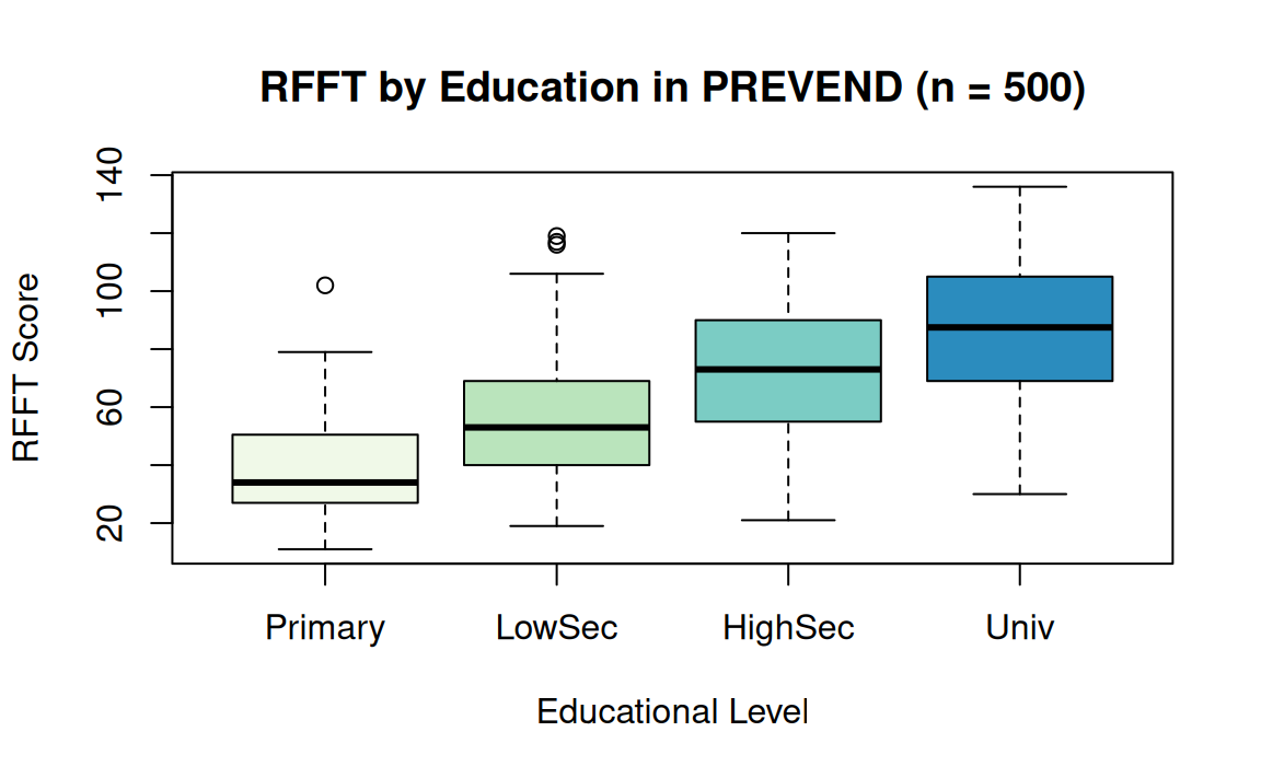
For example: Is RFFT score associated with education?

The variable Education indicates the highest level of education an individual completed in the Dutch educational system:

0: primary school
1: lower secondary school
2: higher secondary education
3: university education

Interpreting regression on `Education`

Baseline category represents individuals who at most completed primary school (Education = 0); Intercept is the sample mean RFFT score for this group.

Coefficients indicates difference in estimated average RFFT relative to baseline group, e.g., predicted increase of 44.96 points for Univ: \(40.94 + 44.96 = 85.90\)

Results of linear regression
	x
(Intercept)	40.94118
EducationLowerSecond	14.77857
EducationHigherSecond	32.13345
EducationUniv	44.96389

Group means
	x
Primary	40.94118
LowerSecond	55.71975
HigherSecond	73.07463
Univ	85.90506

Inference for multiple regression

The coefficients of multiple regression \(\hat{\beta}_0, \hat{\beta}_1, \ldots, \hat{\beta}_p\) are estimates of the population parameters in the regression:

\[y = \beta_0 + \beta_1x_1 + \cdots + \beta_p x_p + \epsilon, \quad \epsilon \sim N(0, \sigma)\]

Inference is usually about slope parameters: \(\beta_1, \beta_2, \dots, \beta_p\)

Typically, the hypotheses of interest are

\(H_0: \beta_k = 0\), the variables \(X_k\) and \(Y\) are not associated
\(H_A: \beta_k \neq 0\), the variables \(X_k\) and \(Y\) are associated

Testing hypotheses about slope coefficients

The \(t\)-statistic has \(df = n - p - 1\), where \(n\) is the sample size and \(p\) is the number of predictors in the model.

\[t = \dfrac{\hat{\beta}_k - \beta_{k, H_0}}{\text{SE}(\hat{\beta}_k)} = \dfrac{\hat{\beta}_k}{\text{SE}(\hat{\beta}_k)}\]

Then, a 95% confidence interval for the slope \(\beta_k\) is given by \[\hat{\beta}_k \pm \left(t^{\star} \times \text{SE}(\hat{\beta}_k) \right),\] where \(t^{\star}\) is the quantile of a \(t\)-distribution with \(n - p - 1\) degrees of freedom with \(\alpha/2\) area to the right.

The \(F\)-statistic in multiple regression

The \(F\)-statistic gives a test (ANOVA) to assess whether predictors in the regression, as a group, are associated with \(Y\).

\(H_0: \beta_1 = \beta_2 = \cdots = \beta_p = 0\)
\(H_A:\) At least one of the slope coefficients is not 0

There is sufficient evidence to reject \(H_0\) (no association) if the \(p\)-value of the \(F\)-statistic is smaller than or equal to \(\alpha\).

summary(lm()) reports the \(F\)-statistic and its \(p\)-value.

Inference: RFFT vs. Education

# model summary
summary(lm(RFFT ~ Education, data = prevend.samp))


Call:
lm(formula = RFFT ~ Education, data = prevend.samp)

Residuals:
    Min      1Q  Median      3Q     Max 
-55.905 -15.975  -0.905  16.068  63.280 

Coefficients:
                      Estimate Std. Error t value Pr(>|t|)    
(Intercept)             40.941      3.203  12.783  < 2e-16 ***
EducationLowerSecond    14.779      3.686   4.009 7.04e-05 ***
EducationHigherSecond   32.133      3.763   8.539  < 2e-16 ***
EducationUniv           44.964      3.684  12.207  < 2e-16 ***
---
Signif. codes:  0 '***' 0.001 '**' 0.01 '*' 0.05 '.' 0.1 ' ' 1

Residual standard error: 22.87 on 496 degrees of freedom
Multiple R-squared:  0.3072,    Adjusted R-squared:  0.303 
F-statistic:  73.3 on 3 and 496 DF,  p-value: < 2.2e-16

# connection to ANOVA
summary(aov(prevend.samp$RFFT ~ prevend.samp$Education))

                        Df Sum Sq Mean Sq F value Pr(>F)    
prevend.samp$Education   3 115041   38347    73.3 <2e-16 ***
Residuals              496 259469     523                   
---
Signif. codes:  0 '***' 0.001 '**' 0.01 '*' 0.05 '.' 0.1 ' ' 1

Reanalyzing the PREVEND data

# fit model adjusting for age, edu, cvd
model1 <- lm(RFFT ~ Statin + Age + Education + CVD, data = prevend.samp)
summary(model1)


Call:
lm(formula = RFFT ~ Statin + Age + Education + CVD, data = prevend.samp)

Residuals:
    Min      1Q  Median      3Q     Max 
-56.348 -15.586  -0.136  13.795  63.935 

Coefficients:
                      Estimate Std. Error t value Pr(>|t|)    
(Intercept)           99.03507    6.33012  15.645  < 2e-16 ***
Statin                 4.69045    2.44802   1.916  0.05594 .  
Age                   -0.92029    0.09041 -10.179  < 2e-16 ***
EducationLowerSecond  10.08831    3.37556   2.989  0.00294 ** 
EducationHigherSecond 21.30146    3.57768   5.954 4.98e-09 ***
EducationUniv         33.12464    3.54710   9.339  < 2e-16 ***
CVDPresent            -7.56655    3.65164  -2.072  0.03878 *  
---
Signif. codes:  0 '***' 0.001 '**' 0.01 '*' 0.05 '.' 0.1 ' ' 1

Residual standard error: 20.71 on 493 degrees of freedom
Multiple R-squared:  0.4355,    Adjusted R-squared:  0.4286 
F-statistic: 63.38 on 6 and 493 DF,  p-value: < 2.2e-16

Interaction in regression

When performing multiple regression, \[y = \beta_0 + \beta_1x_1 + \beta_2x_2 + ... + \beta_px_p + \epsilon\] assumes that a predictor \(x_j\) differing by 1 unit impacts the predicted response by \(\beta_j\), holding other covariates constant.

A statistical interaction describes the case when the impact of an \(x_j\) on the response depends on value(s) of another covariate.

Cholesterol vs. Age and Diabetes

 (Intercept)          Age  DiabetesYes 
 4.800011340  0.007491805 -0.317665963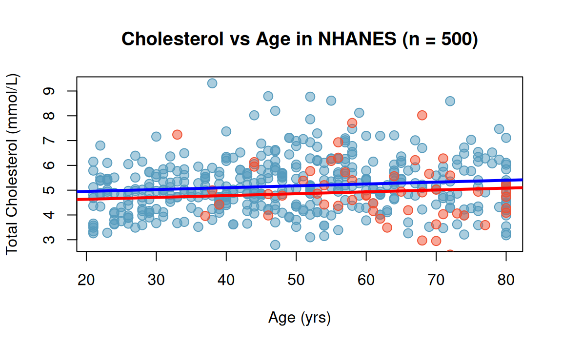

Cholesterol vs. Age and Diabetes

What if two distinct regressions were fit to evaluate total cholesterol and age (varying by diabetic status)?

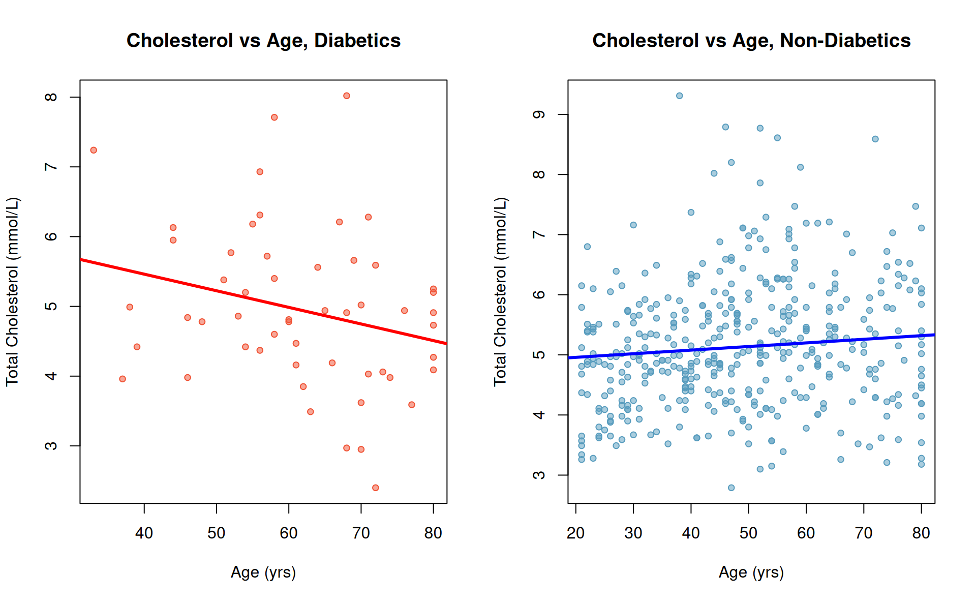
Cholesterol vs. Age and Diabetes

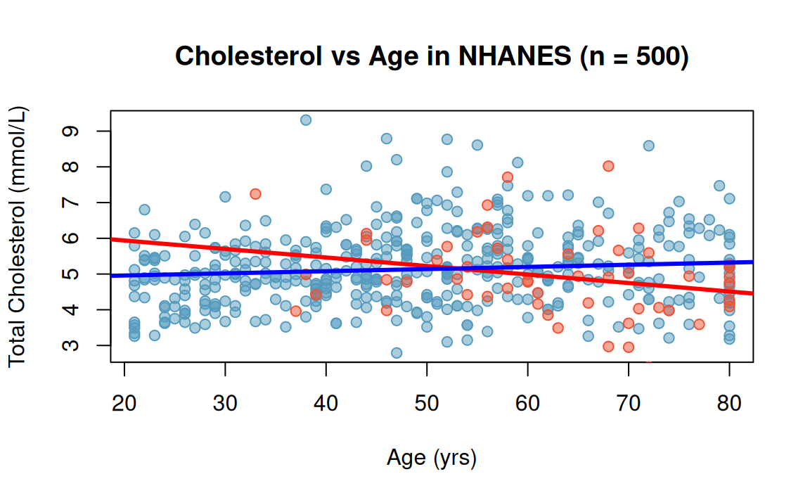
Adding an interaction term

Consider the model \[E(TotChol) = \beta_0 + \beta_1(Age) + \beta_2(Diabetes) + \beta_3(Diabetes \times Age).\]

The term \((Diabetes \times Age)\) is the interaction between diabetes status and age, and \(\beta_3\) is the coefficient of the interaction.

# fit the model
model.interact <- lm(TotChol ~ Age * Diabetes, data = nhanes.samp.adult.500)
coef(model.interact)

    (Intercept)             Age     DiabetesYes Age:DiabetesYes 
    4.695702513     0.009638183     1.718704342    -0.033451562

Significance of an interaction term

summary(model.interact)


Call:
lm(formula = TotChol ~ Age * Diabetes, data = nhanes.samp.adult.500)

Residuals:
    Min      1Q  Median      3Q     Max 
-2.3587 -0.7448 -0.0845  0.6307  4.2480 

Coefficients:
                 Estimate Std. Error t value Pr(>|t|)    
(Intercept)      4.695703   0.159691  29.405  < 2e-16 ***
Age              0.009638   0.003108   3.101  0.00205 ** 
DiabetesYes      1.718704   0.763905   2.250  0.02492 *  
Age:DiabetesYes -0.033452   0.012272  -2.726  0.00665 ** 
---
Signif. codes:  0 '***' 0.001 '**' 0.01 '*' 0.05 '.' 0.1 ' ' 1

Residual standard error: 1.061 on 469 degrees of freedom
  (27 observations deleted due to missingness)
Multiple R-squared:  0.03229,   Adjusted R-squared:  0.0261 
F-statistic: 5.216 on 3 and 469 DF,  p-value: 0.001498

Interpretation: For those with diabetes, increasing age has a negative (not positive!) association with total cholesterol (\(\beta_1 + \beta_3 =\) -0.024)

Comparing nested models

Adding a predictor always increases \(R^2\), so \(R^2\) cannot tell us whether the addition was warranted. The question is a hypothesis test: is the larger model’s improvement in fit larger than chance alone would produce?

For nested linear models, the partial \(F\)-test answers this directly.

# fit a reduced and a full model
mod_reduced <- lm(RFFT ~ Age, data = prevend.samp)
mod_full <- lm(RFFT ~ Age + Education, data = prevend.samp)

# H_0: the Education coefficients are jointly zero
anova(mod_reduced, mod_full)

Analysis of Variance Table

Model 1: RFFT ~ Age
Model 2: RFFT ~ Age + Education
  Res.Df    RSS Df Sum of Sq      F    Pr(>F)    
1    498 267772                                  
2    495 214032  3     53739 41.428 < 2.2e-16 ***
---
Signif. codes:  0 '***' 0.001 '**' 0.01 '*' 0.05 '.' 0.1 ' ' 1

The \(p\)-value tests \(H_0\): every coefficient present only in the full model equals zero. For generalized linear models, anova(..., test = "LRT") performs the analogous likelihood-ratio test.

Logistic regression

A generalization of methods for two-way tables, allowing for joint association between a binary response and several predictors.

Similar in intent to linear regression, but details differ a bit…

the response variable is categorical (specifically, binary)
the model is not estimated via minimizing least squares
the model coefficients have a (very) different interpretation

Survival to discharge in the ICU

Patients admitted to ICUs are very ill — usually from a serious medical event (e.g., respiratory failure, stroke) or from trauma (e.g., traffic accident).

Question: Can patient features available at admission be used to estimate the probability of survival to hospital discharge?

The icu dataset in the aplore3 package is from a study conducted at Baystate Medical Center in Springfield, MA.

The dataset contains information about patient characteristics at admission, including heart rate, diagnosis, kidney function, and much more.
The sta variable includes labels Died (0 for death before discharge) and Lived (1 for survival to discharge).

Survival to discharge in the ICU: To CPR or not?

Let’s take a look at how ICU patients fare with CPR:

        Prior CPR
Survival  No Yes Sum
   Died   33   7  40
   Lived 154   6 160
   Sum   187  13 200

Odds of survival for those who did not receive CPR: \(154/33 = 4.67\)
- \(\text{odds} = \dfrac{p}{1 - p} = \dfrac{0.824}{1 - 0.824} = 4.67\)
Probability of survival for those who did not receive CPR: \(154/187 = 0.824\)
- \(p = \frac{\text{odds}}{1 + \text{odds}} = \dfrac{4.67}{1 + 4.67} = 0.824\)

Odds and probabilities

Probability	Odds = \(p/(1-p)\)	Odds
0	0/1 = 0	0
1/100 = 0.01	1/99 = 0.0101	1 : 99
1/10 = 0.10	1/9 = 0.11	1 : 9
1/4	1/3	1 : 3
1/3	1/2	1 : 2
1/2	\((\frac{1}{2})/(\frac{1}{2})=1\)	1 : 1
2/3	\((2/3)/(1/3)=2\)	2 : 1
3/4	3	3 : 1
1	1/\(0\approx\infty\)	\(\infty\)

Logistic regression

Suppose \(Y\) is a binary variable and \(X\) is a predictor variable.

In our ICU example: \(Y\) is survival to discharge, \(X\) is prior CPR.
Let \(p(x) = \mathbb{P}(Y = 1 \mid X = x)\), for \(Y = 1\) denoting survival.

The model for a single variable logistic regression is \[\log\left[\frac{p(x)}{1 - p(x)}\right] = \beta_0 + \beta_1x\]

Logistic regression models the association between the probability \(p\) of an event of interest and one or more predictor variables.

Why log(odds) in regression models?

Since a probability can only take values from 0 to 1, regression can fail, with the predicted response falling outside the interval \([0,1]\).

The odds, \(p/(1-p)\), ranges from 0 to \(\infty\).
The natural log of the odds (log odds) ranges from \(-\infty\) to \(\infty\).

glm(sta ~ cpr, data = icu, family = binomial(link = "logit"))


Call:  glm(formula = sta ~ cpr, family = binomial(link = "logit"), data = icu)

Coefficients:
(Intercept)       cprYes  
      1.540       -1.695  

Degrees of Freedom: 199 Total (i.e. Null);  198 Residual
Null Deviance:      200.2 
Residual Deviance: 192.2    AIC: 196.2

Interpreting the output

Recall that \(p(x) = \mathbb{P}(Y = 1 \mid X = x) = p(\text{survival = 1} \mid \text{CPR = yes})\).

The logistic regression model’s equation:

\[\log\left[\frac{\hat{p}( \text{status = lived} \mid \text{CPR = yes})}{1 - \hat{p}(\text{status = lived} \mid \text{CPR = yes})}\right] = 1.540 -1.695(\text{CPR = yes})\]

The intercept \(\beta_0\) is the log(\(\widehat{\text{odds}}\) of survival) for ICU patients who didn’t receive CPR:

estimated odds of survival \(= \exp(1.540) = 4.66\)
estimated probability of survival \(= \dfrac{\text{odds}}{\text{1 + odds}} = \dfrac{4.66}{1 + 4.66} = 0.823\)

Interpreting the output…

The slope coefficient \(\beta_1\) of \(\text{CPR = yes}\) represents the difference in log(odds of survival), from the no previous CPR group to the previous CPR group.

The odds of survival in patients who previously received CPR:

\(\log\left[\frac{\hat{p}( \text{status = lived} \mid \text{CPR = yes})}{1 - \hat{p}(\text{status = lived} \mid \text{CPR = yes})}\right] = 1.540 - 1.695(1)\)
\(\widehat{\text{odds}}\) of survival \(= \exp(1.540 - 1.695) = 0.856\)

\(\beta_1\) is the log of the estimated odds ratio for survival, comparing CPR vs. not:

\(\widehat{OR} = \exp(-1.695) = 0.184\)
\(\widehat{OR} = \dfrac{\text{odds}_{\text{CPR = yes}}}{\text{odds}_{\text{CPR = no}}} = \dfrac{0.856}{4.66} = 0.184\)

Inference for simple logistic regression

As with linear regression, the regression slope captures information about the association between a response and a predictor.

\(H_0: \beta_1 = 0\), the \(X\) and \(Y\) variables are not associated
\(H_A: \beta_1 \neq 0\), the \(X\) and \(Y\) variables are associated

These hypotheses can also be written in terms of the odds ratio.

Logistic regression with multiple predictors

Suppose \(p(x) = p(x_1, x_2, \ldots, x_p) = \mathbb{P}(Y = 1 \mid x_1, x_2, \ldots, x_p)\).

With several predictors \(x_1, x_2, \ldots, x_p\) the regression equation is

\[\log\left[\frac{p(x)}{1 - p(x)}\right] = \beta_0 + \beta_1 x_1 + \beta_2 x_2 + \cdots + \beta_p x_p\]

Each coefficient estimates the difference in log(odds) for a one unit difference in that variable, for groups in which the other variables are the same.

Note that this makes \(\exp(\hat{\beta}_k)\) a conditional odds ratio — one computed within groups that share the same values of the other predictors. As we saw when contrasting the relative risk and the odds ratio, this need not match the odds ratio computed while ignoring those other variables, even when none of them is a confounder. This is the non-collapsibility of the odds ratio, and it is a reason to state plainly which odds ratio is being reported.

Survival versus CPR and age

summary(glm(
  sta ~ cpr + cre + age,
  data = icu,
  family = binomial(link = "logit")
))


Call:
glm(formula = sta ~ cpr + cre + age, family = binomial(link = "logit"), 
    data = icu)

Coefficients:
            Estimate Std. Error z value Pr(>|z|)    
(Intercept)  3.32901    0.74884   4.446 8.77e-06 ***
cprYes      -1.69680    0.62145  -2.730  0.00633 ** 
cre> 2.0    -1.13328    0.70191  -1.615  0.10641    
age         -0.02814    0.01125  -2.502  0.01235 *  
---
Signif. codes:  0 '***' 0.001 '**' 0.01 '*' 0.05 '.' 0.1 ' ' 1

(Dispersion parameter for binomial family taken to be 1)

    Null deviance: 200.16  on 199  degrees of freedom
Residual deviance: 181.47  on 196  degrees of freedom
AIC: 189.47

Number of Fisher Scoring iterations: 5

Inference for multiple logistic regression

Typically, the hypotheses of interest are

\(H_0: \beta_k = 0\), the variables \(X_k\) and \(Y\) are not associated
\(H_A: \beta_k \neq 0\), the variables \(X_k\) and \(Y\) are associated

These hypotheses can also be written in terms of the odds ratio.

Regression recap

We considered \(\E[Y \mid X] = \beta_0 + \beta_1 X_1 + \ldots + \beta_p X_p\), the multiple linear regression model with outcome \(Y\) and predictors \(X_1, \ldots, X_p\).

When fitting the regression model, we used ordinary least squares to minimize the sum of squared residuals: \[ (\beta_0, \beta_1, \ldots, \beta_p) = \argmin_{\beta_0, \ldots, \beta_p} \sum_{i=1}^n (y_i - \beta_0 - \beta_1 x_{i1} - \ldots - \beta_p x_{ip})^2 \]
This doesn’t work when the number or predictors exceeds the number of observations, i.e., \(p > n\), in which case the regression problem is ill-posed (an under- or over-determined system of equations).
The case \(p > n\) is a common problem in high-dimensional data analysis.

Regression: Linear and Logistic

Categorical predictors

What about with more than two levels?

Interpreting regression on Education

Inference for multiple regression

Testing hypotheses about slope coefficients

The \(F\)-statistic in multiple regression

Inference: RFFT vs. Education

Reanalyzing the PREVEND data

Interaction in regression

Cholesterol vs. Age and Diabetes

Cholesterol vs. Age and Diabetes

Cholesterol vs. Age and Diabetes

Adding an interaction term

Significance of an interaction term

Comparing nested models

Logistic regression

Survival to discharge in the ICU

Survival to discharge in the ICU: To CPR or not?

Odds and probabilities

Logistic regression

Why log(odds) in regression models?

Interpreting the output

Interpreting the output…

Inference for simple logistic regression

Logistic regression with multiple predictors

Survival versus CPR and age

Inference for multiple logistic regression

Regression recap

Interpreting regression on `Education`