HST 190 at HMS – Introduction to Linear Regression

Regression

Regression methods examine the association between a response variable and a set of possible predictor variables (covariates).

Linear regression posits an approximately linear relationship between the response and predictor variables.
The response variable $y$ can be referred to as the dependent variable, and the predictor variable $x$ the independent variable.
A simple linear regression model takes the form: $Y = β_{0} + β_{1} X + ϵ$

Simple linear regression quantifies how the mean of a response variable $Y$ varies with a single predictor $X$ , assuming linearity.

Multiple regression

Multiple linear regression evaluates the relationship, assuming linearity, between the mean of a response variable, $Y$ , and a vector of predictors, $X_{1}, X_{2}, \dots, X_{p}$ , that is, $Y = β_{0} + β_{1} X_{1} + β_{2} X_{2} + \dots + β_{p} X_{p} + ϵ .$

This is conceptually similar to the simpler case of evaluating $Y$ ’s mean with respect to a single $X$ , except that the interpretation is much more nuanced (more on this later).

Linearity is an approximation; so, think of regression as projection onto a simpler worldview (“if the phenomenon were linear…”).

Back to the PREVEND study

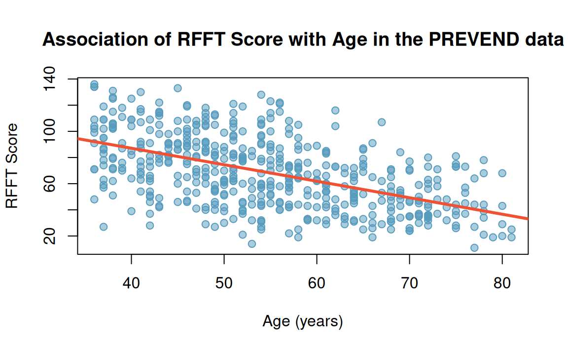
As adults age, cognitive function changes over time, largely due to cerebrovascular and neurodegenerative changes. PREVEND study measured clinical, demographic data for participants, 1997-2006.

Data from 4,095 participants appear the prevend dataset in the oibiostat R package.
Ruff Figural Fluency Test (RFFT) to assess cognitive function (planning and the ability to switch between different tasks).

Assumptions for linear regression

A few assumptions for justifying the use of linear regression to describe how the mean of $Y$ varies with $X$ .

Independent observations: $(x, y)$ pairs are independent; that is, values of one pair provide no information on those of others.
Linearity: $E [Y ∣ X] = f (X)$ is linear and appears justifiably so in the observed data.
Constant variability (homoscedasticity): variability of response $Y$ about the regression line is constant across different values of predictor $X$ .
Approximate normality of residuals: $ϵ \sim N (0, σ_{ϵ}^{2})$

What happens when these assumptions do not hold? 🤔

Linear regression via ordinary least squares

Distance between an observed point $y_{i}$ and the corresponding predicted value ${\hat{y}}_{i}$ from the regression line is the residual for the $i$ ^th unit.

For $(x_{i}, y_{i})$ , where $\hat{y} = {\hat{β}}_{0} + {\hat{β}}_{1} x$ , the residual $e_{i}$ is $e_{i} = y_{i} - {\hat{y}}_{i}$

The least squares regression line minimizes the sum of squared residuals¹ $\sum_{i = 1}^{n} e_{i}^{2}$ among $(x_{i}, y_{i}) \forall i$ to get estimates $({\hat{β}}_{0}, {\hat{β}}_{1})$ .

The mean squared error (MSE), a metric of prediction quality, is also based on the residuals $MSE = \frac{1}{n} \sum_{i = 1}^{n} e_{i}^{2}$ .

Coefficients in least squares linear regression

$β_{0}$ and $β_{1}$ are parameters with estimates ${\hat{β}}_{0}$ and ${\hat{β}}_{1}$ ; estimates can be calculated from summary statistics:

${\hat{β}}_{1} = r \frac{s_{y}}{s_{x}} {\hat{β}}_{0} = \overset{―}{y} - {\hat{β}}_{1} \overset{―}{x}$

$\overset{―}{x}$ , $\overset{―}{y}$ : sample means of $x$ and $y$
$s_{x}$ , $s_{y}$ : sample SD’s of $x$ and $y$
$r$ : correlation between $x$ and $y$

lm(prevend.samp$RFFT ~ prevend.samp$Age)$coef

     (Intercept) prevend.samp$Age 
      137.549716        -1.261359

Least squares regression line $\hat{Y} = {\hat{β}}_{0} + {\hat{β}}_{1} X$ for the association of RFTT and age in the PREVEND data is $\hat{RFFT} = 137.55 - (1.26) (Age)$

Linear regression: The population view

For a population of ordered pairs $(x, y)$ , the population regression line is $Y = β_{0} + β_{1} X + ϵ$ , where $ϵ \sim N (0, σ_{ϵ})$ ¹.

Since $E [ϵ] = 0$ , the regression line is also $E [Y ∣ x] = β_{0} + β_{1} x$ , where $E [Y ∣ x]$ denotes the expectation of $Y$ when $X = x$ .

So, the regression line is a statement about averages: What do we expect the mean of $Y$ to be when $X$ takes on the value $x$ ? If, the mean of $Y$ follows, in fact, a linear relationship in $(β_{0}, β_{1})$ .

Linear regression: Checking assumptions?

Assumptions of linear regression are independence of study units, linearity (in parameters), constant variability, normality of residuals.

Independence should be enforced by well-considered study design.
Other assumptions may be checked empirically…but should we?
- Residual plots: scatterplots in which predicted values are on the $x$ -axis and residuals are on the $y$ -axis
- Normal probability plots: theoretical quantiles for a normal versus observed quantiles (of residuals)
…whether these hold (or not), the claim made is that linearity is a faithful representation of the underlying phenomenon. But is it?

Linear regression with categorical predictors

Although the response variable in linear regression is necessarily numerical, the predictor may be either numerical or categorical.

Simple linear regression only accommodates categorical predictor variables with two levels¹.

Simple linear regression with a two-level categorical predictor $X$ compares the means of the two groups defined by $X$ : $E [Y ∣ X = 1] - E [Y ∣ X = 0] = β_{0} + β_{1} - β_{0} = β_{1}$

Back to FAMuSS: Comparing `ndrm.ch` by sex

Let’s re-examine the association between change in non-dominant arm strength after resistance training and sex in the FAMuSS data.

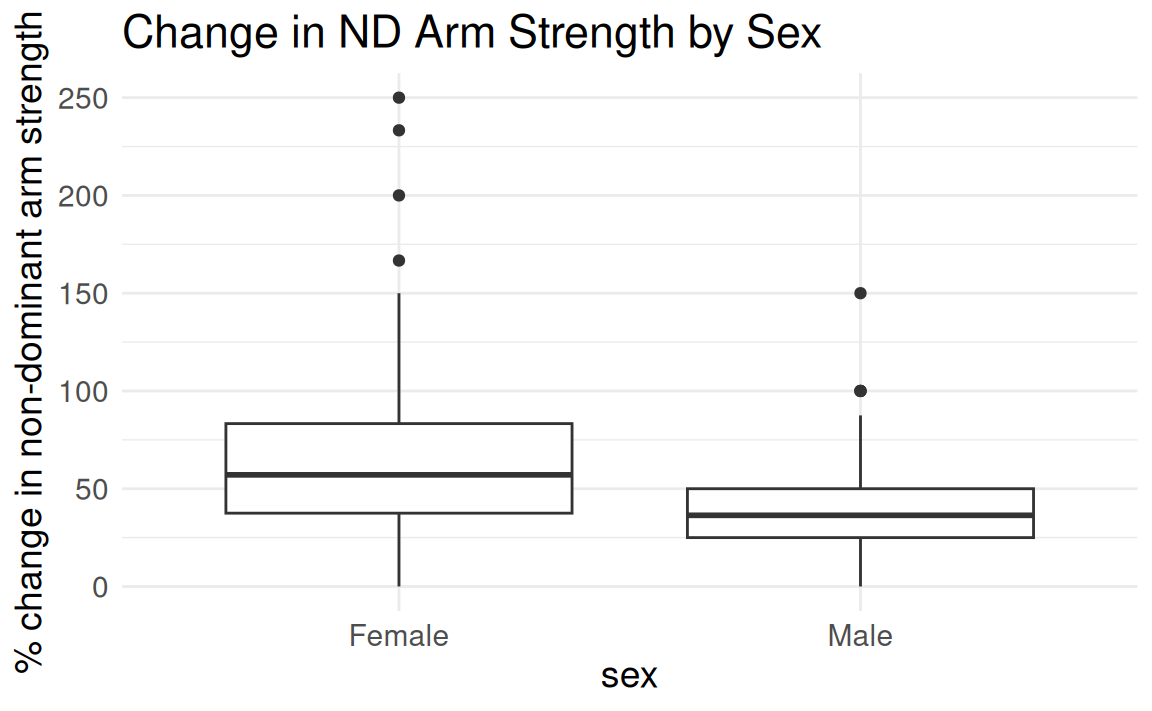
# calculate mean ndrm.ch in each group
tapply(famuss$ndrm.ch, famuss$sex, mean)

  Female     Male 
62.92720 39.23512

# fit a linear model of ndrm.ch by sex
lm(famuss$ndrm.ch ~ famuss$sex)$coef

   (Intercept) famuss$sexMale 
      62.92720      -23.69207

$\hat{ndrm.ch} = 62.93 - 23.59 (sex = male)$

Intercept $β_{0}$ : mean in baseline group
Slope $β_{1}$ : difference of group means

Strength of a regression fit: Using $R^{2}$

Correlation coefficient $r$ measures strength of a linear relationship between $(X, Y)$ ; $r_{X, Y} = Cov (X, Y) / σ_{X} σ_{Y}$ , is the covariance normalized by the SDs
$r^{2}$ (or $R^{2}$ ) more common as a measure of the strength of a linear fit, since $R^{2}$ describes amount of variation in response $Y$ explained by the regression fit

$R^{2} = \frac{Var ({\hat{y}}_{i})}{Var (y_{i})} = \frac{Var (y_{i}) - Var (e_{i})}{Var (y_{i})} = 1 - \sum_{i = 1}^{n} \frac{(y_{i} - {\hat{y}}_{i})^{2}}{(y_{i} - \bar{y})^{2}}$

If a linear regression fit perfectly captured the variability in the observed data, then $Var ({\hat{y}}_{i})$ would equal $Var (y_{i})$ and $R^{2}$ would be 1 (its maximum).
The variability of the residuals about the regression line represents the variability remaining after the fit; $Var (e_{i})$ is the variability unexplained by the regression fit.

Statistical inference in regression

Assume observed data $(x_{i}, y_{i})$ to have been randomly sampled from a population where the explanatory variable $X$ and response variable $Y$ are related as follows $Y = β_{0} + β_{1} X + ϵ, where ϵ \sim N (0, σ_{ϵ}^{2})$

Under this assumption, the slope ${\hat{β}}_{1}$ and intercept ${\hat{β}}_{0}$ of the fitted regression line are estimates of the parameters $β_{0}$ and $β_{1}$ .

Goal: Inference for the slope $β_{1}$ , the association¹ of $X$ with $Y$ .

Hypothesis testing in regression

The null hypothesis $H_{0}$ is most often about no association:

$H_{0} : β_{1} = 0$ , that is, $X$ and $Y$ are not associated
$H_{A} : β_{1} \neq 0$ , that is, $X$ and $Y$ variables are associated

Use the $t$ -test? Recall the $t$ -statistic (here, with $d f = n - 2$ ): $t = \frac{{\hat{β}}_{1} - β_{1, H_{0}}}{SE ({\hat{β}}_{1})} = \frac{{\hat{β}}_{1}}{SE ({\hat{β}}_{1})},$ where $β_{1, H_{0}} = 0$ under the null hypothesis of no association.

Confidence intervals in regression

A $(1 - α)$ (100)% confidence interval for $β_{1}$ is ${\hat{β}}_{1} \pm (t^{⋆} \times SE ({\hat{β}}_{1})),$ where $t^{⋆}$ is the appropriate quantile of a $t$ -distribution, and the standard error¹ of the estimator ${\hat{β}}_{1}$ is $SE (\hat{β}) = \sqrt{\frac{1}{n - 2} \sum_{i = 1}^{n} \frac{(y_{i} - {\hat{y}}_{i})^{2}}{(x_{i} - \bar{x})^{2}}}$

Example: Linear Regression in an RCT

Consider a randomized controlled trial (RCT) that recruits $n = 200$ patients, assigns ( $X$ ) each to drug or placebo, and monitors them until the trial’s end, at which point an outcome $Y$ (e.g., a disease severity score) is measured.

L1	L2	X	Y
1	1	0	1.39
0	0	0	-0.18
0	0	0	-0.20
1	1	1	3.61

The treatment $X$ is randomized, so it will be balanced on the baseline factors (i.e., confounders $L_{1}$ , $L_{2}$ ) on average. Linear regression, $E [Y ∣ X] = β_{0} + β_{1} X$ , gives $E [Y ∣ X = 1] = β_{0} + β_{1} and E [Y ∣ X = 0] = β_{0},$ the difference of which is $E [Y ∣ X = 1] - E [Y ∣ X = 0] = β_{1}$ ¹.

Statistical power and sample size

Question: A collaborator approaches you about this hypothetical RCT, wondering whether $n = 200$ is a sufficient sample size — is it?

In terms of hypothesis testing: $H_{0} : β_{1} = 0$ and $H_{A} : β_{1} > 0$ (the drug “works”). How large does $β_{1}$ have to be for it to be detectable? Is $n = 200$ enough?

The power of a statistical test is the probability that the test (correctly) rejects the null hypothesis $H_{0}$ when the alternative hypothesis $H_{A}$ is true. Power depends on…

the hypothesized effect size ( $β_{1}$ in an RCT – but not generally)
the variance of each of the two groups (i.e., $σ_{1}$ , $σ_{2}$ for treatment, placebo)
the sample sizes of each of the two group ( $n_{1}$ , $n_{2}$ )

Outcomes and errors in testing

	Result of test
State of nature	Reject $H_{0}$	Fail to reject $H_{0}$
$H_{0}$ is true	Type I error, $P = α$ (false positive)	No error, $P = 1 - α$ (true negative)
$H_{A}$ is true	No error, $P = 1 - β$ (true positive)	Type II error, $P = β$ (false negative)

Choosing the right sample size

Study design includes calculating a study size (sample size) such that probability of rejecting $H_{0}$ is acceptably large, typically 80%-90%.

It is important to have a precise estimate of an appropriate study size, since

a study needs to be large enough to allow for sufficient power to detect a difference between groups when one exists, but
not so unnecessarily large that it is cost-prohibitive or unethical.

Often, simulation is a quick and feasible way to conduct a power analysis.

Multiple regression

In most practical settings, more than one explanatory variable is likely to be associated with a response.

Multiple linear regression evaluates the relationship between a response $Y$ and several (say, $p$ ) predictors $X_{1}, X_{2}, \dots, X_{p}$ .

Multiple linear regression takes the form $Y = β_{0} + β_{1} X_{1} + β_{2} X_{2} + \dots + β_{p} X_{p} + ϵ$

PREVEND: Statin use and cognitive function

The PREVEND study collected data on statin use and demographic factors.

Statins are a class of drugs widely used to lower cholesterol.
Recent guidelines for prescribing statins suggest statin use for almost half of Americans 40-75 years old, as well as nearly all men over 60.
A few small (low $n$ ) studies have found evidence of a negative association between statin use and cognitive ability.

Age, statin use, and RFFT score

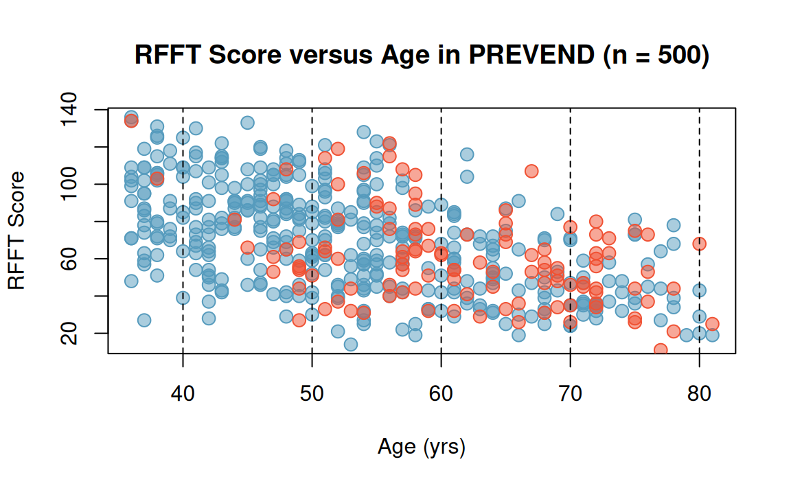
Red dots represent statin users; blue dots represent non-users.


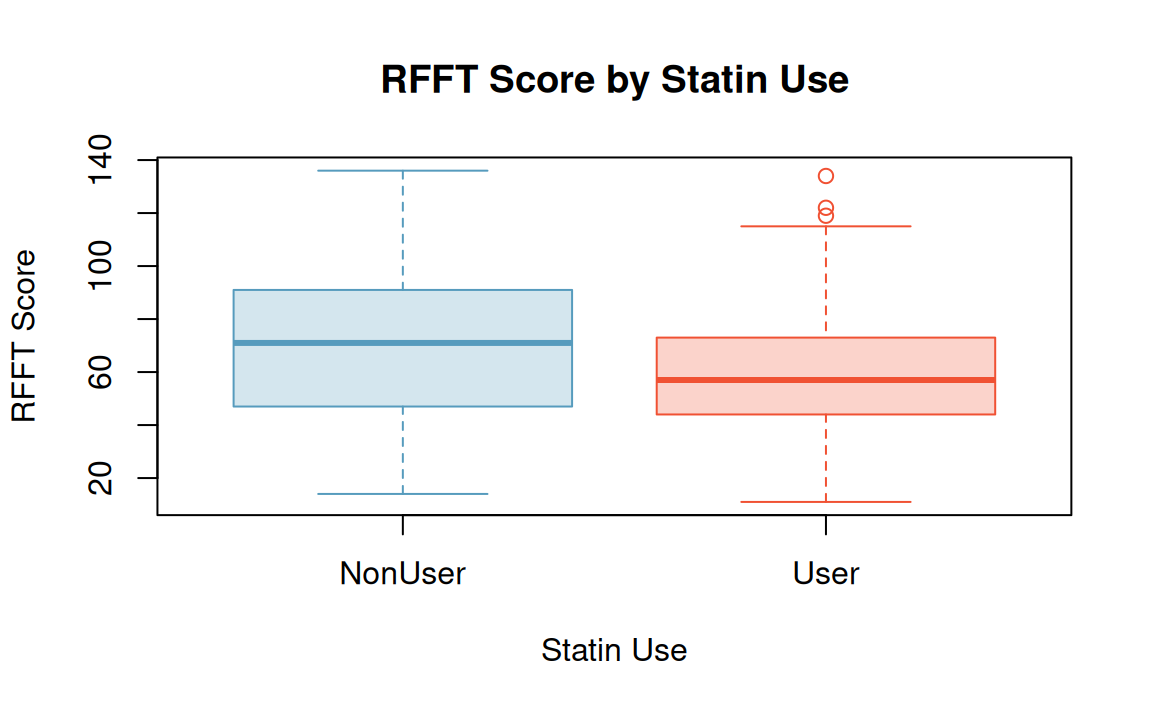
Call:
lm(formula = RFFT ~ Statin, data = prevend.samp)

Coefficients:
(Intercept)   StatinUser  
      70.71       -10.05

Interpretation of regression coefficients

Multiple (linear) regression takes the form $Y = β_{0} + β_{1} X_{1} + β_{2} X_{2} + \dots + β_{p} X_{p} + ϵ,$ where $p$ is the number of predictors (or covariates).

Recall the correspondence of the regression equation with $E [Y ∣ X_{1}, \dots, X_{p}] = β_{0} + β_{1} X_{1} + β_{2} X_{2} + \dots + β_{p} X_{p},$

The coefficient $β_{j}$ of $X_{j}$ : the predicted difference in the mean of $Y$ for groups that differ by one unit in $X_{j}$ and for whom all other predictors take on the same value.

Practically, a coefficient $β_{j}$ in multiple regression is the association between the response $Y$ and predictor $X_{j}$ , after adjusting for other predictors $X_{i} : i = 1, \dots, p | i \neq j$ .

In action: RFFT vs. statin use and age

Fit the multiple regression with lm():

# fit the linear model
prevend_multreg <- lm(RFFT ~ Statin + Age, data = prevend.samp)
prevend_multreg


Call:
lm(formula = RFFT ~ Statin + Age, data = prevend.samp)

Coefficients:
(Intercept)   StatinUser          Age  
   137.8822       0.8509      -1.2710

$β_{statin} =$ 0.851 — so it seems statin use is associated with a positive difference in RFTT, when adjusting for age (i.e., for study units in the same age range).

# print the model summary for the coefficients
summary(prevend_multreg)$coef |> round(3)

            Estimate Std. Error t value Pr(>|t|)
(Intercept)  137.882      5.122  26.919    0.000
StatinUser     0.851      2.596   0.328    0.743
Age           -1.271      0.094 -13.478    0.000

Assumptions for multiple regression

Analogous to those of simple linear regression…

Independence: units $(y_{i}, x_{1, i}, x_{2, i}, \dots, x_{p, i})$ independent in $i$ .
Linearity: for each predictor variable $x_{j}$ , difference in the predictor is linearly related to difference in the response variable in groups defined by all other predictors taking on the same value.
Constant variability: $ϵ$ have approximately constant variance.
Normality of residuals: $ϵ$ approximately normally distributed.

References

Tsiatis, Anastasios A, Marie Davidian, Min Zhang, and Xiaomin Lu. 2008. “Covariate Adjustment for Two-Sample Treatment Comparisons in Randomized Clinical Trials: A Principled yet Flexible Approach.” Statistics in Medicine 27 (23): 4658–77. https://doi.org/10.1002/sim.3113.