
Regression: Linear, Logistic, Regularized
September 3, 2025
Categorical predictors
With a binary predictor, linear regression estimates the difference in the mean response between groups defined by the levels.
For example, the equation for linear regression of RFFT score from statin use with the data prevend.samp is \[\widehat{\text{RFFT}} = 70.71 - 10.05(\text{StatinUser})\]
- Mean RFFT score for individuals not using statins is 70.71.
- Mean RFFT score for individuals using statins is 10.05 points lower than non-users, \(70.71 - 10.05 = 60.66\).
What about with more than two levels?
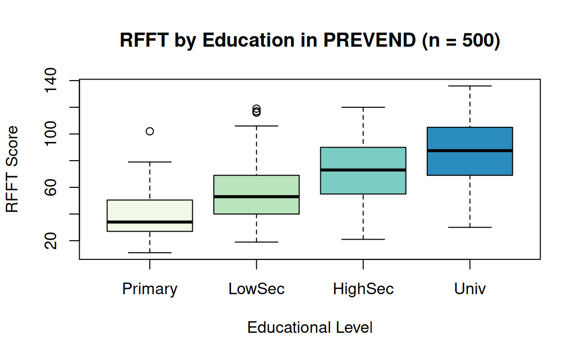
For example: Is RFFT score associated with education?
The variable Education indicates the highest level of education an individual completed in the Dutch educational system:
- 0: primary school
- 1: lower secondary school
- 2: higher secondary education
- 3: university education
Interpreting regression on Education
Baseline category represents individuals who at most completed primary school (Education = 0); Intercept is the sample mean RFFT score for this group.
Coefficients indicates difference in estimated average RFFT relative to baseline group, e.g., predicted increase of 44.96 points for Univ: \(40.94
+ 44.96 = 85.90\)
| x | |
|---|---|
| (Intercept) | 40.94118 |
| EducationLowerSecond | 14.77857 |
| EducationHigherSecond | 32.13345 |
| EducationUniv | 44.96389 |
| x | |
|---|---|
| Primary | 40.94118 |
| LowerSecond | 55.71975 |
| HigherSecond | 73.07463 |
| Univ | 85.90506 |
Inference for multiple regression
The coefficients of multiple regression \(\hat{\beta}_0, \hat{\beta}_1, \ldots, \hat{\beta}_p\) are estimates of the population parameters in the regression:
\[y = \beta_0 + \beta_1x_1 + \cdots + \beta_p x_p + \epsilon, \quad \epsilon \sim N(0, \sigma)\]
Inference is usually about slope parameters: \(\beta_1, \beta_2, \dots, \beta_p\)
Typically, the hypotheses of interest are
- \(H_0: \beta_k = 0\), the variables \(X_k\) and \(Y\) are not associated
- \(H_A: \beta_k \neq 0\), the variables \(X_k\) and \(Y\) are associated
Testing hypotheses about slope coefficients
The \(t\)-statistic has \(df = n - p - 1\), where \(n\) is the sample size and \(p\) is the number of predictors in the model.
\[t = \dfrac{\hat{\beta}_k - \beta_{k, H_0}}{\text{SE}(\hat{\beta}_k)} = \dfrac{\hat{\beta}_k}{\text{SE}(\hat{\beta}_k)}\]
Then, a 95% confidence interval for the slope \(\beta_k\) is given by \[\hat{\beta}_k \pm \left(t^{\star} \times \text{SE}(\hat{\beta}_k) \right),\] where \(t^{\star}\) is the quantile of a \(t\)-distribution with \(n - p - 1\) degrees of freedom with \(\alpha/2\) area to the right.
The \(F\)-statistic in multiple regression
The \(F\)-statistic gives a test (ANOVA) to assess whether predictors in the regression, as a group, are associated with \(Y\).
- \(H_0: \beta_1 = \beta_2 = \cdots = \beta_p = 0\)
- \(H_A:\) At least one of the slope coefficients is not 0
There is sufficient evidence to reject \(H_0\) (no association) if the \(p\)-value of the \(F\)-statistic is smaller than or equal to \(\alpha\).
summary(lm()) reports the \(F\)-statistic and its \(p\)-value.
Inference: RFFT vs. Education
Call:
lm(formula = RFFT ~ Education, data = prevend.samp)

Residuals:
    Min      1Q  Median      3Q     Max
-55.905 -15.975  -0.905  16.068  63.280

Coefficients:
                      Estimate Std. Error t value Pr(>|t|)
(Intercept)             40.941      3.203  12.783  < 2e-16 ***
EducationLowerSecond    14.779      3.686   4.009 7.04e-05 ***
EducationHigherSecond   32.133      3.763   8.539  < 2e-16 ***
EducationUniv           44.964      3.684  12.207  < 2e-16 ***
---
Signif. codes:  0 '***' 0.001 '**' 0.01 '*' 0.05 '.' 0.1 ' ' 1

Residual standard error: 22.87 on 496 degrees of freedom
Multiple R-squared:  0.3072,    Adjusted R-squared:  0.303
F-statistic: 73.3 on 3 and 496 DF, p-value: < 2.2e-16Reanalyzing the PREVEND data
# fit model adjusting for age, edu, cvd
model1 <- lm(RFFT ~ Statin + Age + Education + CVD,
             data = prevend.samp)
summary(model1)
Call:
lm(formula = RFFT ~ Statin + Age + Education + CVD, data = prevend.samp)

Residuals:
    Min      1Q  Median      3Q     Max
-56.348 -15.586  -0.136  13.795  63.935

Coefficients:
                      Estimate Std. Error t value Pr(>|t|)
(Intercept)           99.03507    6.33012  15.645  < 2e-16 ***
Statin                 4.69045    2.44802   1.916  0.05594 .
Age                   -0.92029    0.09041 -10.179  < 2e-16 ***
EducationLowerSecond  10.08831    3.37556   2.989  0.00294 **
EducationHigherSecond 21.30146    3.57768   5.954 4.98e-09 ***
EducationUniv         33.12464    3.54710   9.339  < 2e-16 ***
CVDPresent            -7.56655    3.65164  -2.072  0.03878 *
---
Signif. codes:  0 '***' 0.001 '**' 0.01 '*' 0.05 '.' 0.1 ' ' 1

Residual standard error: 20.71 on 493 degrees of freedom
Multiple R-squared:  0.4355,    Adjusted R-squared:  0.4286
F-statistic: 63.38 on 6 and 493 DF,  p-value: < 2.2e-16
Interaction in regression
When performing multiple regression, \[y = \beta_0 + \beta_1x_1 + \beta_2x_2 + ... + \beta_px_p + \epsilon\] assumes that a predictor \(x_j\) differing by 1 unit impacts the predicted response by \(\beta_j\), holding other covariates constant.
A statistical interaction describes the case when the impact of an \(x_j\) on the response depends on value(s) of another covariate.
Cholesterol vs. Age and Diabetes
 (Intercept)          Age  DiabetesYes
4.800011340 0.007491805 -0.317665963 
Cholesterol vs. Age and Diabetes
What if two distinct regressions were fit to evaluate total cholesterol and age (varying by diabetic status)?
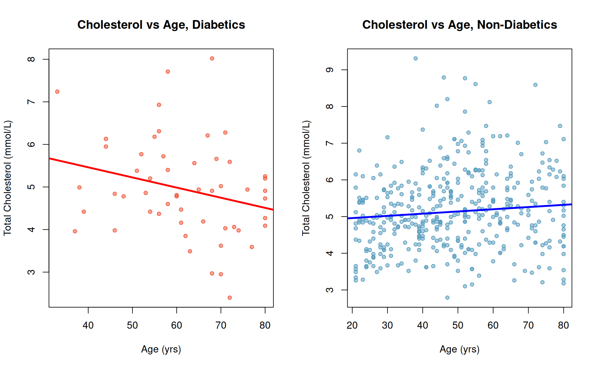
Cholesterol vs. Age and Diabetes
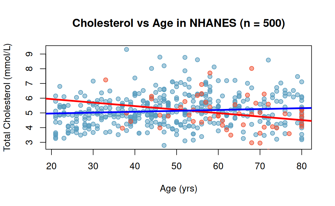
Adding an interaction term
Consider the model \[E(TotChol) = \beta_0 + \beta_1(Age) + \beta_2(Diabetes) + \beta_3(Diabetes \times Age).\]
The term \((Diabetes \times Age)\) is the interaction between diabetes status and age, and \(\beta_3\) is the coefficient of the interaction.
Significance of an interaction term
Call:
lm(formula = TotChol ~ Age * Diabetes, data = nhanes.samp.adult.500)

Residuals:
    Min      1Q  Median      3Q     Max
-2.3587 -0.7448 -0.0845  0.6307  4.2480

Coefficients:
                 Estimate Std. Error t value Pr(>|t|)
(Intercept)      4.695703   0.159691  29.405  < 2e-16 ***
Age              0.009638   0.003108   3.101  0.00205 **
DiabetesYes      1.718704   0.763905   2.250  0.02492 *
Age:DiabetesYes -0.033452   0.012272  -2.726  0.00665 **
---
Signif. codes:  0 '***' 0.001 '**' 0.01 '*' 0.05 '.' 0.1 ' ' 1

Residual standard error: 1.061 on 469 degrees of freedom
  (27 observations deleted due to missingness)
Multiple R-squared:  0.03229,   Adjusted R-squared:  0.0261
F-statistic: 5.216 on 3 and 469 DF,  p-value: 0.001498
Interpretation: For those with diabetes, increasing age has a negative (not positive!) association with total cholesterol (\(\beta_1 + \beta_3 =\) -0.024)
\(R^2\) with multiple regression
As in simple regression, \(R^2\) represents the proportion of variability in the response variable explained by the model.
As variables are added, \(R^2\) always increases.
In the summary(lm()) output, Multiple R-squared is \(R^2\).
Adjusted \(R^2\) as a tool for model assessment
\[R_{adj}^{2} = 1 - \left( \frac{\text{Var}(e_i)}{\text{Var}(y_i)} \times \frac{n-1}{n-p-1} \right),\] where \(n\) is the number of units and \(p\) is the number of predictors.
Adjusted \(R^2\) incorporates a penalty for the inclusion of predictors that fail to contribute much to explaining observed variation in \(Y\).
- often used to balance predictive ability and model complexity.
- unlike \(R^2\), \(R^2_{adj}\) does not have an inherent interpretation.
Logistic regression
A generalization of methods for two-way tables, allowing for joint association between a binary response and several predictors.
Similar in intent to linear regression, but details differ a bit…
- the response variable is categorical (specifically, binary)
- the model is not estimated via minimizing least squares
- the model coefficients have a (very) different interpretation
Survival to discharge in the ICU
Patients admitted to ICUs are very ill — usually from a serious medical event (e.g., respiratory failure, stroke) or from trauma (e.g., traffic accident).
Question: Can patient features available at admission be used to estimate the probability of survival to hospital discharge?
The icu dataset in the aplore3 package is from a study conducted at Baystate Medical Center in Springfield, MA.
- The dataset contains information about patient characteristics at admission, including heart rate, diagnosis, kidney function, and much more.
- The
stavariable includes labelsDied(0for death before discharge) andLived(1for survival to discharge).
Survival to discharge in the ICU: To CPR or not?
Let’s take a look at how ICU patients fare with CPR:
        Prior CPR
Survival  No Yes Sum
   Died   33   7  40
   Lived 154   6 160
Sum 187 13 200- Odds of survival for those who did not receive CPR: \(154/33 = 4.67\)
- \(\text{odds} = \dfrac{p}{1 - p} = \dfrac{0.824}{1 - 0.824} = 4.67\)
- Probability of survival for those who did not receive CPR: \(154/187 =
0.824\)
- \(p = \frac{\text{odds}}{1 + \text{odds}} = \dfrac{4.67}{1 + 4.67} = 0.824\)
Odds and probabilities
| Probability | Odds = \(p/(1-p)\) | Odds |
|---|---|---|
| 0 | 0/1 = 0 | 0 |
| 1/100 = 0.01 | 1/99 = 0.0101 | 1 : 99 |
| 1/10 = 0.10 | 1/9 = 0.11 | 1 : 9 |
| 1/4 | 1/3 | 1 : 3 |
| 1/3 | 1/2 | 1 : 2 |
| 1/2 | \((\frac{1}{2})/(\frac{1}{2})=1\) | 1 : 1 |
| 2/3 | \((2/3)/(1/3)=2\) | 2 : 1 |
| 3/4 | 3 | 3 : 1 |
| 1 | 1/\(0\approx\infty\) | \(\infty\) |
Logistic regression
Suppose \(Y\) is a binary variable and \(X\) is a predictor variable.
- In our ICU example: \(Y\) is survival to discharge, \(X\) is prior CPR.
- Let \(p(x) = \mathbb{P}(Y = 1 \mid X = x)\), for \(Y = 1\) denoting survival.
The model for a single variable logistic regression is \[\log\left[\frac{p(x)}{1 - p(x)}\right] = \beta_0 + \beta_1x\]
Logistic regression models the association between the probability \(p\) of an event of interest and one or more predictor variables.
Why log(odds) in regression models?
Since a probability can only take values from 0 to 1, regression can fail, with the predicted response falling outside the interval \([0,1]\).
- The odds, \(p/(1-p)\), ranges from 0 to \(\infty\).
- The natural log of the odds (log odds) ranges from \(-\infty\) to \(\infty\).
Interpreting the output
Recall that \(p(x) = \mathbb{P}(Y = 1 \mid X = x) = p(\text{survival = 1} \mid \text{CPR = yes})\).
The logistic regression model’s equation:
\[\log\left[\frac{\hat{p}( \text{status = lived} \mid \text{CPR = yes})}{1 - \hat{p}(\text{status = lived} \mid \text{CPR = yes})}\right] = 1.540 -1.695(\text{CPR = yes})\]
The intercept \(\beta_0\) is the log(\(\widehat{\text{odds}}\) of survival) for ICU patients who didn’t receive CPR:
- estimated odds of survival \(= \exp(1.540) = 4.66\)
- estimated probability of survival \(= \dfrac{\text{odds}}{\text{1 + odds}} = \dfrac{4.66}{1 + 4.66} = 0.823\)
Interpreting the output…
The slope coefficient \(\beta_1\) of \(\text{CPR = yes}\) represents the difference in log(odds of survival), from the no previous CPR group to the previous CPR group.
The odds of survival in patients who previously received CPR:
- \(\log\left[\frac{\hat{p}( \text{status = lived} \mid \text{CPR = yes})}{1 - \hat{p}(\text{status = lived} \mid \text{CPR = yes})}\right] = 1.540 - 1.695(1)\)
- \(\widehat{\text{odds}}\) of survival \(= \exp(1.540 - 1.695) = 0.856\)
\(\beta_1\) is the log of the estimated odds ratio for survival, comparing CPR vs. not:
- \(\widehat{OR} = \exp(-1.695) = 0.184\)
- \(\widehat{OR} = \dfrac{\text{odds}_{\text{CPR = yes}}}{\text{odds}_{\text{CPR = no}}} = \dfrac{0.856}{4.66} = 0.184\)
Inference for simple logistic regression
As with linear regression, the regression slope captures information about the association between a response and a predictor.
- \(H_0: \beta_1 = 0\), the \(X\) and \(Y\) variables are not associated
- \(H_A: \beta_1 \neq 0\), the \(X\) and \(Y\) variables are associated
These hypotheses can also be written in terms of the odds ratio.
Logistic regression with multiple predictors
Suppose \(p(x) = p(x_1, x_2, \ldots, x_p) = \mathbb{P}(Y = 1 \mid x_1, x_2, \ldots, x_p)\).
With several predictors \(x_1, x_2, \ldots, x_p\) the regression equation is
\[\log\left[\frac{p(x)}{1 - p(x)}\right] = \beta_0 + \beta_1 x_1 + \beta_2 x_2 + \cdots + \beta_p x_p\]
Each coefficient estimates the difference in log(odds) for a one unit difference in that variable, for groups in which the other variables are the same.
Survival versus CPR and age
Call:
glm(formula = sta ~ cpr + cre + age, family = binomial(link = "logit"),
    data = icu)

Coefficients:
            Estimate Std. Error z value Pr(>|z|)
(Intercept)  3.32901    0.74884   4.446 8.77e-06 ***
cprYes      -1.69680    0.62145  -2.730  0.00633 **
cre> 2.0    -1.13328    0.70191  -1.615  0.10641
age         -0.02814    0.01125  -2.502  0.01235 *
---
Signif. codes:  0 '***' 0.001 '**' 0.01 '*' 0.05 '.' 0.1 ' ' 1

(Dispersion parameter for binomial family taken to be 1)

    Null deviance: 200.16  on 199  degrees of freedom
Residual deviance: 181.47  on 196  degrees of freedom
AIC: 189.47

Number of Fisher Scoring iterations: 5
Inference for multiple logistic regression
Typically, the hypotheses of interest are
- \(H_0: \beta_k = 0\), the variables \(X_k\) and \(Y\) are not associated
- \(H_A: \beta_k \neq 0\), the variables \(X_k\) and \(Y\) are associated
These hypotheses can also be written in terms of the odds ratio.
Regression recap
We considered \(\E[Y \mid X] = \beta_0 + \beta_1 X_1 + \ldots + \beta_p X_p\), the multiple linear regression model with outcome \(Y\) and predictors \(X_1, \ldots, X_p\).
- When fitting the regression model, we used ordinary least squares to minimize the sum of squared residuals: \[ (\beta_0, \beta_1, \ldots, \beta_p) = \argmin_{\beta_0, \ldots, \beta_p} \sum_{i=1}^n (y_i - \beta_0 - \beta_1 x_{i1} - \ldots - \beta_p x_{ip})^2 \]
- This doesn’t work when the number or predictors exceeds the number of observations, i.e., \(p > n\), in which case the regression problem is ill-posed (an under- or over-determined system of equations).
- The case \(p > n\) is a common problem in high-dimensional data analysis.
Regularized regression
- In this high-dimensional setting, how do we choose the relevant predictors to fit the best model that we can?
- A penalized or regularized regression procedure changes the quantity we minimize to discourage choosing too many variables.
- Force estimates of \(\beta\) for unimportant predictors to zero, excluding these from the chosen model
- Regularized regression is a general family of procedures involving different forms of penalization, including lasso, ridge, and elastic net.
Regularized regression: Ridge
The ridge (or Tikhonov) regularized regression estimator minimizes a sum of squares subject to an \(L_2\) (squared) penalty on the \(\beta_j\). It is defined
\[ (\tilde{\beta}_0, \tilde{\beta}_1, \ldots, \tilde{\beta}_p) = \argmin_{\beta_0, \ldots, \beta_p} \left(\sum_{i=1}^n (y_i - \beta_0 - \beta_1 x_{i1} - \ldots - \beta_p x_{ip})^2 + \lambda \sum_{j=1}^p \beta_j^2 \right) \ . \]
- The penalty (degree of regularization) is set by the tuning parameter \(\lambda\).
- As \(\lambda\) is increased, the ridge penalty shrinks estimated coefficients towards zero slowly, leaving many variables in the model.
- The choice of \(\lambda\) determines the selected regression model, so how do we go about choosing \(\lambda\)?
Regularized regression: Lasso
The lasso regularized regression estimator minimizes a sum of squares subject to an \(L_1\) (absolute) penalty on the \(\beta_j\). It is defined
\[ (\tilde{\beta}_0, \tilde{\beta}_1, \ldots, \tilde{\beta}_p) = \argmin_{\beta_0, \ldots, \beta_p} \left(\sum_{i=1}^n (y_i - \beta_0 - \beta_1 x_{i1} - \ldots - \beta_p x_{ip})^2 + \lambda \sum_{j=1}^p \lvert \beta_j \rvert \right) \ . \]
- Again, the penalty (degree of regularization) is controlled by the tuning parameter \(\lambda\).
- As \(\lambda\) is increased, the lasso penalty shrinks estimated coefficients towards zero, setting many to zero exactly.
- There are many variations to the lasso (group lasso, fused lasso, etc.), and it is a popular variable selection strategy.
Regularized regression: Elastic net
The elastic net regularized regression estimator combines the ridge and lasso penalties. It is defined as
\[ (\tilde{\beta}_0, \tilde{\beta}_1, \ldots, \tilde{\beta}_p) = \argmin_{\beta_0, \ldots, \beta_p} \left(\sum_{i=1}^n (y_i - \beta_0 - \beta_1 x_{i1} - \ldots - \beta_p x_{ip})^2 + \lambda_1 \sum_{j=1}^p \lvert \beta_j \rvert + \lambda_2 \sum_{j=1}^p \beta_j^2 \right) \ . \]
- Note the correspondence to ridge regression (when \(\lambda_1 = 0\)) and also to lasso regression (when \(\lambda_2 = 0\)).
- The elastic net overcomes some pitfalls of the lasso, including that the lasso can fail to isolate a best predictor from among a group of related predictors, with the \(L_2\) penalty ensuring a unique minimum.
Generalization in regression
Regression methods borrow information across \(X\) to learn about the form of the regression function \(\E[Y \mid X]\) via some selected model.
- How do we choose \(X\) to include, or, equivalently, how do we choose \(\lambda\) in regularized regression?
- Borrowing (or smoothing) across all \(X\) to inform \(\E[Y \mid X]\), regression is a global learning problem (for \(X_j = x\), \(\beta_j\) is fixed).
- borrowing too much across \(X\) leads to high bias
- borrowing too little across \(X\) leads to high variance
- the goal is to find the right balance: bias-variance trade-off
- Can we use the available data to make an optimal choice of \(\lambda\)?
Generalization in regression
What if we evaluate a large collection (e.g., in \(\lambda\)) of pre-specified regression techniques, choosing the best one as our final estimate \(\hat{\E}[Y \mid X]\)?
- we can still entirely pre-specify the whole estimation procedure
- …but we need to determine how to pick the best technique
Can we run a fair competition between estimators to determine the best? If so, how would we go about doing this?
Cross-validation and generalization
How can we estimate the risk of an estimator?
Idea: Use empirical risk estimate \[ \hat{R}(\hat{\E})(X) = \frac{1}{n}\sum_{i=1}^n \left\{Y_i - \hat{\E}(X_i)\right\}^2 \]
Problem: \(\hat{\E}(\cdot)\) would fitted using the same data that we use to estimate its risk! (We’re testing the estimator on training data.)
Cross-validation and generalization
By analogy: A student got a glimpse of the exam before taking it.
- focused on learning test questions very well…but
- test result doesn’t reflect how well student learned the subject
With \(n=100\) units, fit linear regression \(X + X^2 + \dots + X^{20}\) \[ \hat{\E}(x) = \hat{\beta}_0 + \hat{\beta}_1 x + + \hat{\beta}_2 x^2 + \cdots + \hat{\beta}_{20} x^{20} \] versus fitting the true, unknown linear regression, say, \(X + X^2 + X^3\) \[ \hat{\E}(x) = \hat{\beta}_0 + \hat{\beta}_1 x + \hat{\beta}_2 x^2 + \hat{\beta}_3 x^3 \]
Cross-validation and generalization
When we use the same data to fit the regression function and to evaluate it:
- we are overly optimistic about how well each estimator is fit;
- so, we would select the wrong estimator.
What we need is external data to properly evaluate estimators.
- We could get a better idea of how well estimators are doing.
- We could objectively select the correct estimator to use.
- …but such data are rarely available.
Cross-validation
Instead, we use cross-validation to estimate the risk.
- Fit regression on part of the data, evaluate on another part.
- Mimics the evaluation of the given fit on external data.
- Many forms of cross-validation1: \(V\)-fold cross-validation is a simple and very popularly used scheme.
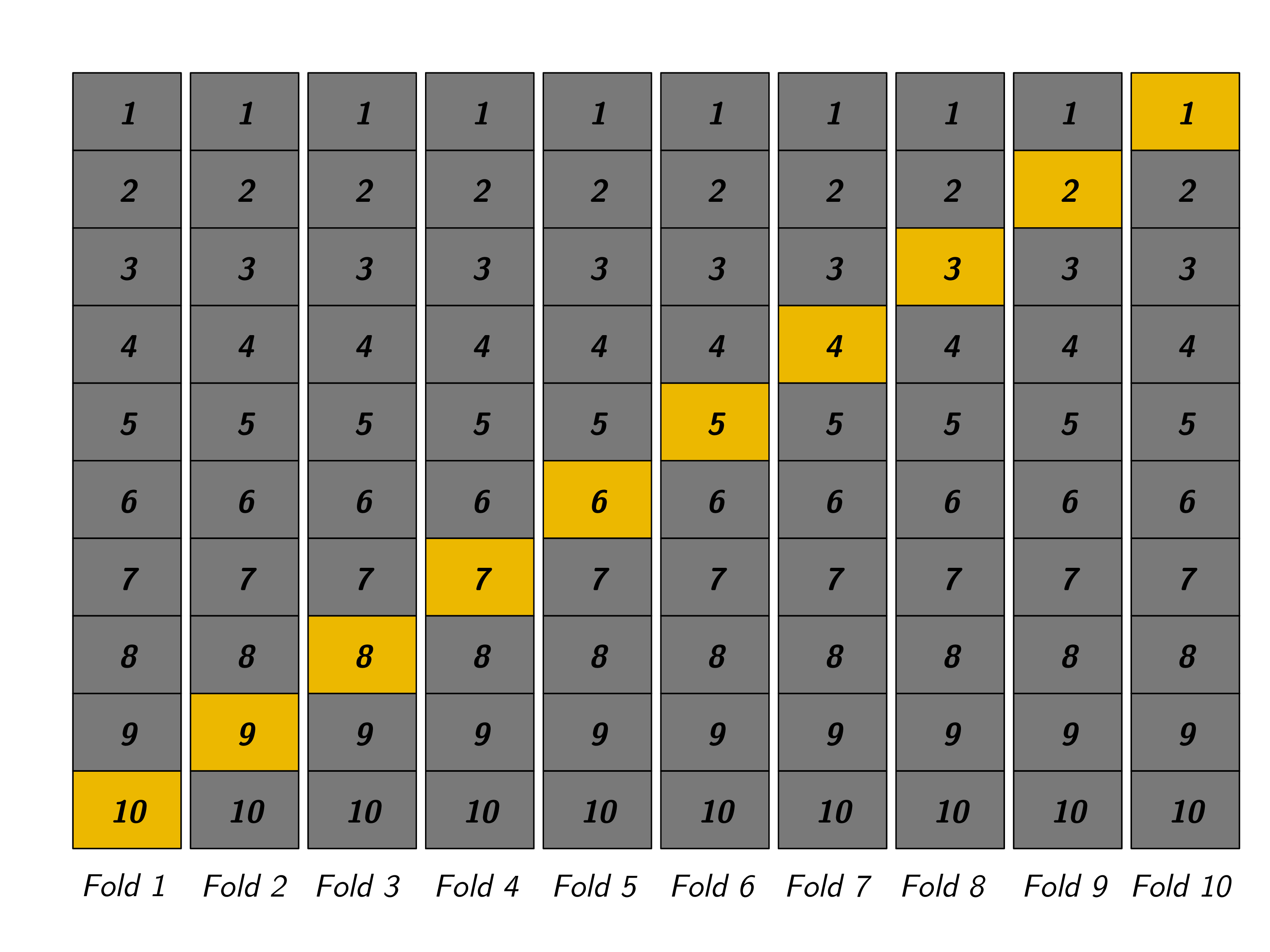
Cross-validation
Data are divided into \(V\) sets of size \(\approx \frac{n}{V}\). Here, \(V=10\).
- Training sample is used to fit (“train”, “learn”) the regressions.
- Validation sample is used to estimate risk (“validate”, “test”, “evaluate”).
Several factors to consider when choosing \(V\):
- large \(V\) = more data to fit regressions1; greater computation time
- small \(V\) = more data to evaluate risk2;

HST 190: Introduction to Biostatistics