Survival Analysis
Introduction to the analysis of time-to-event data

September 3, 2025
Survival analysis?
Survival analysis is studied distinctly from other topics since survival data have some important distinguishing features.
Nonetheless, our tour of survival analysis will (re)visit many of the topics we have already learned considered so far
- estimation
- one-sample inference
- two-sample inference
- regression
Survival analysis is the area of (bio)statistics that deals with time-to-event data.
Survival analysis?
“Survival” analysis isn’t restricted to analyzing time until death: Applicable whenever the time until study subjects experience a relevant endpoint is of interest.
The terms “failure” and “event” are used interchangeably for the endpoint of interest.
Example: Researchers record time from diagnosis until death for a sample of patients diagnosed with laryngeal cancer.
- How would you summarize the survival of these patients?
- Which of the summary measures discussed thus far seem appropriate or applicable?
Summarizing survival data
What if the mean or median survival time were reported?
- The sample mean is not robust to outliers: Did everyone live a little bit longer or just a few people live a lot longer?
- The median is just a summary measure: If considering your own prognosis, you’d want to know more!
What if survival rate at \(x\) years were reported?
- How to choose the cutoff time \(x\)? (1 year, 5 years…)
- Also, still just a single summary measure…
Measuring survival times
Denote the measured time by the RV \(T\), and let \(t=0\) be the beginning of the period being studied (e.g., time of diagnosis).
Time is recorded relative to when a person enters the study, not according to the calendar.
- A study unit reaches \(t=1\) after being in the study for one year (or month, day, etc.)
- Time is relative to a given unit’s own entry into the study: It doesn’t matter how far along others are
Measuring survival times
The probability of an individual in our population surviving past a given time \(t\) is given by the survival function \(S(t)\)
Here, we are interested in inference about a function, not just a single population value (e.g., \(\mu\))
Can we estimate \(S(t)\) by taking a random sample and recording the proportion of study units still alive after time \(t\) has elapsed?
- If only it was as simple as it sounds…
When data go missing: Censoring
Analyses of survival times usually include censored/missing data; valid inference with missing data is a topic of ongoing research in statistics – generally, assumptions are required.
Time-to-event data exhibit a particular form of missingness: units are lost to follow-up (or the study ends) prior to their experiencing the event of interest; this is called right-censoring.
Censored data provide partial information: we don’t know how long a patient lived, but we know they lived at least as long as the time elapsed prior to being lost to follow-up.
The censoring problem
Why would a person be lost to follow-up? They could have…
- moved to another city
- withdrawn from the study
- died of a different cause
- still be in the study without an event at time of analysis
Critical assumption: Censoring is non-informative—that is, assume that being lost to follow-up is unrelated to prognosis. (Is this plausible?)
If this assumption can’t be made, inference becomes more complicated and requires strong(er) assumptions.
The censoring problem
Counterexample: Researchers administer a new chemotherapy drug to 10 cancer patients to assess survival while on the drug.
- 5 patients can’t tolerate the side effects, drop out of study
- Those who dropped out were likely more ill—thus, shorter survival times disproportionately removed from the sample (bias?)
If non-informative censoring were assumed, the drug would probably appear falsely impressive.
Estimating the survival curve
The Kaplan-Meier estimator (Kaplan and Meier 1958) gives an estimate of \(S(t)\) at all \(t\), even when some data are censored
For specific times \(t_1, \ldots, t_k\), the KM estimator at \(t_j\) is \[ \begin{align*} S(t_j) &= \P(\text{alive at } t_j) \\ &= \P(\text{alive at } t_j \cap \text{alive at } t_{j-1}) \\ &= \P(\text{alive at } t_j \mid \text{alive at } t_{j-1}) \cdot \P(\text{alive at } t_{j-1}) \\ &= \P(\text{alive at } t_j \mid \text{alive at } t_{j-1}) \cdot S(t_{j-1}) \end{align*} \]
Probability of surviving to time \(t_j\) is the probability of surviving to \(t_{j-1}\) and, then, given making it that far, surviving to \(t_j\).
What if we applied this recursive trick repeatedly?
Estimating the survival curve
Survival function \(S(t)\) at time \(t\) expressed in terms of past survival: \[ \begin{align*} S(t_j) &= \mathbb{P}(\text{alive at } t_j \mid \text{alive at } t_{j-1}) \cdot S(t_{j-1}) \\ &= \mathbb{P}(\text{alive at } t_{j-1}) \cdot \mathbb{P}(\text{alive at } t_{j-1} \mid \text{alive at } t_{j-2}) \cdot S(t_{j-2}) \\ &= \mathbb{P}(\text{alive at } t_j \mid \text{alive at } t_{j-1}) \ldots \mathbb{P}(\text{alive at } t_2 \mid \text{alive at } t_1) \cdot S(t_1) \end{align*} \]
Without censoring: \(\mathbb{P}(\text{alive at } t_j \mid \text{alive at } t_{j-1}) \approx \dfrac{\# \text{alive at } t_j}{\# \text{alive at } t_{j-1}}\)
Note: a patient alive but censored at \(t_{j-1}\) never really made it to \(t_j\)
- That patient was not eligible to die during the interval from \(t_{j-1}\) to \(t_j\) and therefore shouldn’t be counted for computing survival rate in this interval
- When a patient (study unit) is ineligible to die during a given interval, we say that that patient is not in the risk set
Estimating the survival curve
Under censoring, we estimate \(\mathbb{P}(\text{alive at } t_j \mid \text{alive at } t_{j−1})\) using its sample analog: \[ \dfrac{\# \text{alive at } t_j}{\# \text{alive at } t_{j-1} - \# \text{censored at } t_{j-1}} \]
Denominator counts those at risk for the event at time \(t_j\) (“risk set”)
With independent censoring, we can invoke the logic of conditional probability: \(\mathbb{P}(\text{alive at } t_j \mid \text{alive at } t_{j-1} \text{and uncensored at } t_j)\)
Estimating the survival curve
For convenience, define the following quantities
- \(d_j = \#\) died at time \(t_j\)
- \(l_j = \#\) censored at time \(t_j\)
- \(S_j = \#\) still alive and not censored at \(t_j\)
Now, notice that \(S_{j-1} = S_j + d_j + l_j\), so we have \[ \begin{align*} \dfrac{\# \text{alive at } t_j}{\# \text{alive at } t_{j-1} - \# \text{censored at } t_{j-1}} &= \dfrac{S_j + l_j}{S_{j-1} + l_{j-1} - l_{j-1}} \\&= \dfrac{S_{j - 1} - d_j}{S_{j-1}} = 1 - \dfrac{d_j}{S_{j-1}} \end{align*} \]
Estimating the survival curve
From this, at observed times \(t_1, \ldots, t_k\), the Kaplan-Meier (KM) estimator of the survival probability at time \(t_j\) is \[ \begin{align*} \hat{S}(t_j) &= \left(1 - \dfrac{d_1}{S_0}\right) \cdot \left(1 - \dfrac{d_2}{S_1}\right) \cdot \ldots \cdot \left(1 - \dfrac{d_j}{S_{j-1}}\right)\\ &= \prod_{k=1}^j \left(1 - \dfrac{d_k}{S_{k-1}}\right) \end{align*} \]
- Estimated survival curve \(\hat{S}(t_j)\) jumps at event times only
- \(\hat{S}(t_j)\) goes to zero only if the last observed event time is an uncensored event
Estimating the survival curve: Worked example
Consider \(n = 100\) patients with outcomes measured at 2-year intervals:
year fail censored 2 7 2 4 16 5 6 19 8 8 14 7 10 11 4 12 5 2
Computing estimates survival probabilities with the KM estimator just applies the formula:
- \(\hat{S}(2) = 1 - \dfrac{7}{100} = 0.93\)
- \(\hat{S}(4) = \left(1 - \frac{7}{100}\right) \cdot \left(1 - \dfrac{16}{91}\right) = 0.77\)
- \(\hat{S}(6) = \left(1 - \dfrac{7}{100}\right) \cdot \left(1 - \dfrac{16}{91}\right) \cdot \left(1 - \dfrac{19}{70}\right) = 0.56\)
- and so on…
The Kaplan-Meier Estimator
\[ \begin{align*} \hat{S}(t_j) &= \left(1 - \dfrac{d_1}{S_0}\right) \cdot \left(1 - \dfrac{d_2}{S_1}\right) \cdot \ldots \cdot \left(1 - \dfrac{d_j}{S_{j-1}}\right)\\ &= \prod_{k=1}^j \left(1 - \dfrac{d_k}{S_{k-1}}\right) \end{align*} \]
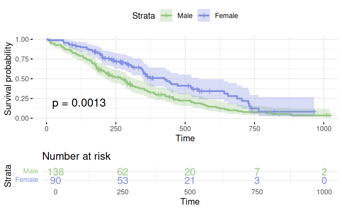
Estimated survival curves – in action!
Inference for the Kaplan-Meier estimator
Estimating \(S(t)\) at any time point \(t_j\) isn’t enough…we also want inference (e.g., confidence intervals) for it as well.
Using a log-transformation for this improves upon the normal approximation. A step-by-step sketch:
- Take logarithm of \(S(t)\)
- Confidence interval (CI) for \(\log(S(t))\)
- Convert back to CI for \(S(t)\) by exponentiating
Inference for the Kaplan-Meier estimator
- At \(t_j\), the variance1 is \(\text{Var}[\log(\hat{S}(t_j))] = \sum_{k=1}^j \dfrac{d_k}{S_{k-1} (S_{k-1} - d_k)}\)
- So, at a given time \(t_j\), the \((1 - \alpha)(100)\)% CI for \(\log(S(t_j))\) is \[\log(\hat{S}(t_j)) \pm z_{1 - \alpha/2} \sqrt{\sum_{k=1}^j \dfrac{d_k}{S_{k-1} (S_{k-1} - d_k)}} = (c_1, c_2)\]
- So, the \((1 - \alpha)(100)\)% CI for \(S(t_j)\) is \((\exp(c_1), \exp(c_2))\)
- In our example: \(\hat{S}(6) = 0.558 \implies \log(\hat{S}(6)) = -0.583\)
Inference for the Kaplan-Meier estimator
- Then, applying Greenwood’s formula, \(\text{Var}(\log(\hat{S}(6)))\) is \[\begin{align*} \sum_{k=1}^j& \dfrac{d_k}{S_{k-1} (S_{k-1} - d_k)} = \dfrac{d_1}{S_0 (S_0 - d_1)} + \dfrac{d_2}{S_1 (S_1 - d_2)} + \dfrac{d_3}{S_2 (S_2 - d_3)} \\ &= \dfrac{7}{100 (100 - 7)} + \dfrac{16}{91 (91 - 16)} + \dfrac{19}{70 (70 - 19)} = 0.008 \end{align*}\]
- And the \((1 - \alpha)(100)\)% CIs for \(\log(\hat{S}(6))\) and \(\hat{S}(6)\), respectively, are \[\begin{align*} -0.583 \pm 1.96 \sqrt{0.008} &= (-0.763, -0.403) \\ (\exp(-0.763), \exp(-0.403)) &= (0.466, 0.668) \end{align*}\]
Hypothesis testing: The log-rank test
In addition to estimating survival, we may want to compare two groups’ survival functions formally (i.e., via a hypothesis test).
Rather than testing for differences in a summary measure (e.g., mean in groups 1 vs. 2), we compare the entire survival curves.
- The test for this is called the Log-Rank Test.
- But what does it mean to say “two curves are the same”?
To precisely define what we’re testing, we need to define a new function called the hazard function, \(h(t)\) (often \(\lambda(t)\)).
Interlude: The hazard function
The hazard function \(h(t)\) is defined as \[\begin{align*} h(t) &= \dfrac{\lim_{\Delta t \to 0} \dfrac{S(t) - S(t + \Delta t)} {\Delta t}}{S(t)} \\ &= \dfrac{\text{instantaneous death rate per unit time}} {\text{proportion of individuals still alive}} \end{align*}\]
Equivalently, this is the instantaneous conditional event rate
In discrete time, this is the probability of an event occurring at time \(t\), given no event has occurred up to time \(t\)
Interlude: Hazard to survival (and back again…)
Special relationships of the survival function \(S(t) = \mathbb{P}(T > t)\):
\[ \begin{align*} h(t) &= \dfrac{\lim_{\Delta t \to 0} \dfrac{S(t) - S(t + \Delta t)} {\Delta t}}{S(t)} \quad \text{and} \quad H(t) = \int_0^t h(\tau) d\tau \\ S(t) &= \exp(-H(t)) = \exp\left(-\int_0^t h(\tau) d\tau\right) \quad \text{and} \quad F(t) = 1 - S(t) \,\, \end{align*} \] \(h(t)\): the hazard function, \(H(t)\): the cumulative hazard function, \(S(t)\): the survival function, \(F(t)\): the (lifetime) distribution function
See Freedman (2008) for an overview of these critical relationships.
The log-rank test
Hazard functions are natural constructs for handling censoring.
Formulate null and alternative hypotheses to test whether two groups have different survival functions based on the hazard:
- \(H_0: h_1(t) = h_2(t)\) for all \(t\) during the study
- \(H_A: h_1(t) \neq h_2(t)\) at some point during the study
The log-rank test subdivides time into \(k\) intervals, and, for each interval (or event time), constructs a \(2 \times 2\) table (“death or no death” vs. “exposure or no exposure”)1
Regression (is all you need?)
For continuous outcomes (\(Y \in \mathbb{R}\)), we formulated linear regression as \(y = \beta_0 + \beta_1 x_1 + \ldots + \beta_k x_k + \epsilon\)
For binary outcomes (\(Y \in \{0, 1\}\)), we formulated logistic regression as \(\log\left(\dfrac{p(x)}{1 - p(x)}\right) = \beta_0 + \beta_1 x_1 + \ldots + \beta_k x_k\)
What about for survival data? Any ideas?
- What is the outcome that we observe? \(T \in (0, \infty)\)
- A failure time (\(T_F\))? A censoring time (\(T_C\))? Both?
- Not quite: The minimum of these, i.e., \(T = \min(T_F, T_C)\)
The Cox model: Regression (is all you need?)
Survival curves don’t necessarily follow a given distribution…
- Sometimes a distribution will be assumed, but inference can be seriously distorted if the distribution is not correct.
- Is the survival time really exponential, Weibull, etc.?
Cox’s proportional hazards model is a special semiparametric regression heavily used in survival analysis (Cox 1972).
Assumption: hazard \(h(t)\) is a function of covariates \(X_1, \ldots, X_k\): \[ \begin{align*} h(t) &= h_0(t) \exp(\beta_1 x_1 + \ldots + \beta_k x_k) \\ \log\left(\dfrac{h(t)}{h_0(t)}\right) &= \beta_1 x_1 + \ldots + \beta_k x_k \end{align*} \]
The Cox model: Regression (is all you need?)
In this regression model, \(h_0(t)\) is called the baseline hazard rate.
Given hazard rate \(h(t)\), and holding all else constant, what is the associational impact of a single unit change of \(X_1\)? \[ \begin{align*} h_{\text{old}}(t) &= h_0(t) \exp(\beta_1 x_1 + \ldots + \beta_k x_k) \implies \\ h_{\text{new}}(t) &= h_0(t) \exp(\beta_1 (1 + x_1) + \ldots + \beta_k x_k) \\ &= \exp(\beta_1) \cdot h_0(t) \exp(\beta_1 x_1 + \ldots + \beta_k x_k) = \exp(\beta_1) \cdot h_{\text{old}}(t) \end{align*} \]
Proportional hazards: Unit change in covariate \(x_j\) should change the hazard by a constant proportionally (if the model holds).
We’ve said nothing about the baseline hazard rate \(h_0(t)\) – we make no assumptions about it, estimating it nonparametrically.
References

HST 190: Introduction to Biostatistics